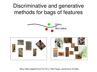
Discriminative and generative classifiers

1. Discriminative and generativeclassifiers Mei-Chen Yeh May 1, 2012

2. Outline • Discriminative classifiers for image recognition • Boosting (last time) • Nearest neighbors (+ scene match app) • Support vector machines • Generative classifiers • Naïve bayes • Part-based models Partial slide credits are from Martin Law and K. Grauman

3. Lines in R2 Let distance from point to line

4. Linear classifiers • Find linear function to separate positive and negative examples How many lines we may have to separate the data? Which lineis best?

5. Formulation • Given training data: (xi, yi), i = 1, 2, …, N • xi: feature vector • yi: label • Learn a hyper-plane which separates all data • variables: w and w0 • Testing: decision function f(x) = sign(g(x)) = sign(wTx + w0) • x: unseen data

6. H2 H3 Class 2 H1 Class 1 Hyperplanes H1, H2, and H3 are candidate classifiers. Which one is preferred? Why?

7. Choose the one with large margin! Class 2 Class 2 Class 1 Class 1

8. margin? Distance between point and line: Class 2 For points on the boundaries: wTx + w0 = δ 1 wTx + w0 = 0 wTx + w0 = -δ -1 scale w, w0 so that Class 1

9. Formulation • Compute w, w0 so that to: The decision boundary should classify all points correctly! Side information:

10. Formulation • The problem is equal to the optimization task: • w can be recovered by Lagrange multipliers

11. Remarks • Just some λ are not zeros. • xiwith non-zero λ are called support vectors. • The hyperplane is determined only by the support vectors. Class 2 Class 1

12. Remarks • For testing an unseen data z • The cost function is in the form of inner products. • does not depend explicitly on the dimensionality of the input space! Class 2 Class 1

13. A geometric interpretation λ = 0 λ = 0.6 w λ = 0.2 λ = 0 λ = 0 λ = 0 λ = 0.8 λ = 0 λ = 1.4 λ = 0 λ = 0 wTx + w0 = 0 Non-separable Cases?

14. Formulation 2: Non-separable Classes Allow training errors! Previous constraint: yi(wTxi+ w0) ≥ 1 Class 2 Introduce errors: yi(wTxi+ w0) ≥ 1- ξi • ξi> 1 • 0 < ξi≤ 1 Class 1 • others, ξi= 0

15. Formulation (cont.) tradeoff between the error and the margin • Compute w, w0 so that to:

16. Formulation (cont.) • The dual form: • w can be recovered by • The only difference with the linearly separable case is that there is an upper bound C onλi

17. Questions • What if the data is not linearly separable? • What if we have more than just two categories?

18. x 0 x 0 x2 Non-linear SVMs • Datasets that are linearly separable with some noise work out great: • But what are we going to do if the dataset is just too hard? • How about… mapping data to a higher-dimensional space: 0 x

19. Non-linear SVMs: feature spaces • General idea: the original input space can be mapped to some higher-dimensional feature space where the training set is separable: Φ: x→φ(x) Slide from Andrew Moore’s tutorial: http://www.autonlab.org/tutorials/svm.html

20. f( ) f( ) f( ) f( ) f( ) f( ) f( ) f( ) f( ) f( ) f( ) f( ) f( ) f( ) f( ) f( ) f( ) f( ) Non-linear SVMs • Example: f(.)

21. Problems • High computation burden • Hard to get a good estimate

22. Kernel Trick • Recall that w can be recovered by All we need here is the inner product of (transformed) feature vectors!

23. Kernel Trick • Decision function • A kernel function is a similarity function that corresponds to an inner product in some expanded feature space. • K(xi, xj) = f(xi)Tf(xj)

24. Example kernel The inner product can be directly computed without going through the mapping f(.)

25. Remarks • In practice, we specify K(x, y), thereby specifying f(.) indirectly, instead of choosing f(.). • Intuitively, K(x, y) represents our desired notion of similarity between data x and y and this is from our prior knowledge. • K(x, y) needs to satisfy a technical condition (Mercer condition)in order for f(.) to exist.

26. Examples of kernel functions • Linear: • Gaussian RBF: • Histogram intersection: Research on different kernel functions in different applications is very active!

27. SVMs: Pros and cons • Pros • Many publicly available SVM packages:http://www.csie.ntu.edu.tw/~cjlin/libsvm/ • Kernel-based framework is very powerful, flexible • Often a sparse set of support vectors – fast testing • Work very well in practice, even with very small training sample sizes • Cons • No “direct” multi-class SVM, must combine two-class SVMs • Can be tricky to select a good kernel function for a problem • Computation, memory • During training time, must compute matrix of kernel values for every pair of examples • Learning can take a very long time for large-scale problems Adapted from Lana Lazebnik

28. Questions • What if the data is not linearly separable? • What if we have more than just two categories?

29. Multi-class SVMs • Achieve multi-class classifier by combining a number of binary classifiers • One vs. all • Training: learn an SVM for each class vs. the rest • Testing: apply each SVM to test example and assign to it the class of the SVM that returns the highest decision value SVM_1/23 SVM_2/13 SVM_3/12 class 1 class 2 class 3

30. Multi-class SVMs • Achieve multi-class classifier by combining a number of binary classifiers • One vs. one • Training: learn an SVM for each pair of classes • Testing: each learned SVM “votes” for a class to assign to the test example SVM_1/3 SVM_1/2 SVM_2/3 class 1 class 2 class 3

31. Data normalization • The features may have different ranges. Example: We use weight (w) and height (h) for classifying male and female college students. • male: avg.(w) = 69.80 kg, avg.(h) = 174.36 cm • female: avg.(w) = 52.86 kg, avg.(h) = 159.77 cm Features with large values may have a larger influence in the cost function than features with small values.

32. Data normalization • “Data pre-processing” • Equalize scales among different features • Zero mean and unit variance • Two cases in practice • (0, 1) if all feature values are positive • (-1, 1) if feature values may be positive or negative

33. Data normalization • xik: feature k, sample i, • Mean and variance • Normalization back

34. SVMs: Summary • Two key concepts of SVM: maximize the margin and the kernel trick • Many SVM implementations are available on the web for you to try on. • LIBSVM: http://www.csie.ntu.edu.tw/~cjlin/libsvm/