CS546: Machine Learning and Natural Language Discriminative vs Generative Classifiers
280 likes | 493 Vues
CS546: Machine Learning and Natural Language Discriminative vs Generative Classifiers. This lecture is based on (Ng & Jordan, 02) paper and some slides are based on Tom Mitchell’s slides. TexPoint fonts used in EMF. Read the TexPoint manual before you delete this box.: A. Outline.

CS546: Machine Learning and Natural Language Discriminative vs Generative Classifiers
E N D
Presentation Transcript
CS546: Machine Learning and Natural LanguageDiscriminative vs Generative Classifiers This lecture is based on (Ng & Jordan, 02) paper and some slides are based on Tom Mitchell’s slides TexPoint fonts used in EMF. Read the TexPoint manual before you delete this box.: A
Outline • Reminder: Naive Bayes and Logistic Regression (MaxEnt) • Asymptotic Analysis • What is better if you have an infinite dataset? • Non-asymptotic Analysis • What is the rate of convergence of parameters? • More important: convergence of the expected error • Empirical evaluation • Why this lecture? • Nice and simple application of Large Deviation bounds we considered before • We will analyze specifically NB vsLogRegression, but “hope” it generalizes to other models (e.g, models for sequence labeling or parsing)
Discriminative vs Generative • Training classifiers involves estimating f: X Y, or P(Y|X) • Discriminative classifiers (conditional models) • Assume some functional form for P(Y|X) • Estimate parameters of P(Y|X) directly from training data • Generative classifiers (joint models) • Assume some functional form for P(X|Y), P(X) • Estimate parameters of P(X|Y), P(X) directly from training data • Use Bayes rule to calculate P(Y|X= xi)
Naive Bayes • Example: assume Y boolean, X = <x1, x2, …, xn>, where xi are binary • Generative model: Naive Bayes • Classify new example x based on ratio • You can do it in log-scale s indicates size of set. l is smoothing parameter
Naive Bayes vs Logistic Regression • Generative model: Naive Bayes • Classify new example x based on ratio • Logistic Regression: • Recall: both classifiers are linear
What is the difference asymptotically? • Notation: let denote error of hypothesis learned via algorithm A, from m examples • If the Naive Bayes model is true: • Otherwise • Logistic regression estimator is consistent: • ² (hDis,m) converges to • H is the class of all linear classifers • Therefore, it is asymptotically better than the linear classifier selected by the NB algorithm
Rate of covergence: logistic regression • Convergences to best linear classifier, in order of n examples • follows from Vapnik’s structural risk bound (VC-dimension of n dimensional linear separators is n+1 )
Rate of covergence: Naive Bayes • We will proceed in 2 stages: • Consider how fast parameters converge to their optimal values • (we do not care about it, actually) • We care: Derive how it corresponds to the convergence of the error to the asymptotical error • The authors consider a continous case (where input is continious) but it is not very interesting for NLP • However, similar techniques apply
Proof of Lemma (no smoothing for simplicity) • By the Chernoff’s bound, with probability at least : • the fraction of positive examples will be within of : • Therefore we have at least positive and negative examples • By the Chernoff’s bound for every feature and class label (2n cases) with probability • We have one event with probability and 2n events with probabilities , there joint probability is not greater than sum: • Solve this for m, and you get
Implications • With a number of samples logarithmic in n (not linear as for the logistic regression!) the parameters of approach parameters of • Are we done? • Not really: this does not automatically imply that • the error approaches with the same rate
Implications • We need to show that and “often” agree if their parameters are close • We compare log-scores given by the models: and • I.e.:
Convergence of Classifiers • G – defines the fraction of points very close to the decision boundary • What is this fraction? See later
Proof of Theorem (sketch) • By the lemma (with high probability) the parameters of are within : of those of • It implies that every term in the sum is also within • of the term in and hence • Let • So and can have different predictions only if • Probability of this event is
Convergence of Classifiers • G -- What is this fraction? • This is somewhat more difficult
Convergence of Classifiers • G -- What is this fraction? • This is somewhat more difficult
What to do with this theorem • This is easy to prove, no proof but intuition: • A fraction of terms in have large expectation • Therefore, the sum has also large expectation
What to do with this theorem • But this is weaker then what we need: • We have that the expectation is “large” • We need that the probability of small values is low • What about Chebyshev inequality? • They are not independent ... How to deal with it?
Corollary from the theorem • Is this condition realistic? • Yes (e.g., we can show it for rather realistic conditions)
Empirical Evaluation (UCI dataset) • Dashed line is logistic regression • Solid line is Naives Bayes
Empirical Evaluation (UCI dataset) • Dashed line is logistic regression • Solid line is Naives Bayes
Empirical Evaluation (UCI dataset) • Dashed line is logistic regression • Solid line is Naives Bayes
Summary • Logistic regression has lower asymptotic error • ... But Naive Bayes needs less data to approach its asymptotic error
First Assignment • I am still checking it, I will let you know by/on Friday • Note though: • Do not perform multiple tests (model selection) on the final test set! • It is a form of cheating
Term Project / Substitution • This Friday I will distribute the first phase -- due after the Spring break • I will be away for the next 2 weeks: • the first week (Mar, 9 – Mar, 15): I will be slow to respond to email • I will be substituted for this week by: • Active Learning (Kevin Small) • Indirect Supervision (Alex Klementiev) • Presentation by Ryan Cunningham on Friday • week Mar, 16 - Mar, 23 – no lectures: • work on the project, send questions if needed
