Random variables, distributions and limit theorems
Random variables, distributions and limit theorems. Gil McVean, Department of Statistics Wednesday 11 th February 2009. Questions to ask…. What is a random variable? What is a distribution? Where do ‘commonly-used’ distributions come from? What distribution does my data come from?

Random variables, distributions and limit theorems
E N D
Presentation Transcript
Random variables, distributions and limit theorems Gil McVean, Department of Statistics Wednesday 11th February 2009
Questions to ask… • What is a random variable? • What is a distribution? • Where do ‘commonly-used’ distributions come from? • What distribution does my data come from? • Do I have to specify a distribution to analyse my data?
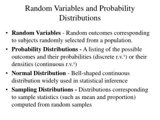
What is a random variable? • A random variable is a number associated with the outcome of a stochastic process • Waiting time for next bus • Average number hours sunshine in May • Age of current prime-minister • In statistics, we want to take observations of random variables and use this to make statements about the underlying stochastic process • Did this vaccine have any effect? • Which genes contribute to disease susceptibility? • Will it rain tomorrow? • Parametric models provide much power in the analysis of variation (parameter estimation, hypothesis testing, model choice, prediction) • Statistical models of the random variables • Models of the underlying stochastic process
x x What is a distribution? • A distribution characterises the probability (mass) associated with each possible outcome of a stochastic process • Distributions of discrete data characterised by probability mass functions • Distributions of continuous data are characterised by probability density functions (pdf) • For RVs that map to the integers or the real numbers, the cumulative density function (cdf)is a useful alternative representation 0 1 2 3
Some notation conventions • Instances of random variables (RVs) are usually written in uppercase • Values associated with RVs are usually written in lowercase • pdfs are often written as f(x) • cdfs are often written as F(x) • Parameters are often defined asq • Hence Probability that the ith random variable takes value x given sample size n and parameter(s) q The probability density associated with outcome x given some parameter(s) q
Expectations and variances • Suppose we took a large sample from a particular distribution, we might want to summarise something about what observations look like ‘on average’ and how much variability there is • The expectation of a distribution is the average value of a random variable over a large number of samples • The variance of a distribution is the average squared difference between randomly sampled observations and the expected value
iid • In most cases, we assume that the random variables we observe are independent and identically distributed • The iid assumption allows us to make all sorts of statements both about what we expect to see and how much variation to expect • Suppose X, Y and Z are iid random variables and a and b are constants
Where do ‘commonly-used’ distributions come from? • At the core of much statistical theory and methodology lie a series of key distributions (e.g. Normal, Poisson, Exponential, etc.) • These distributions are closely related to each other and can be ‘derived’ as the limit of simple stochastic processes when the random variable can be counted or measured • In many settings, more complex distributions are constructed from these ‘simple’ distributions • Ratios: E.g. Beta, Cauchy • Compound: E.g. Geometric, Beta • Mixture models
An aside on Chebyshev’s inequality • Let X be a random variable with mean m and variance s2 • Chebyshev’s inequality states that for any t > 0 • This allows us to make statements about any distribution with finite variance • The probability that a value lies more than 2 standard deviations from the mean is less than or equal to 0.25 • Note that this is an upper bound. In reality, the distribution might be considerably tighter • E.g. for the normal distribution the probability is 0.046, for the exponential distribution the probability is 0.05
The simplest model • Bernoulli trials • Outcomes that can take only two values: (0 and 1) with probabilities q and 1 - qrespectively. E.g. coin flipping, indicator functions • The likelihood function calculates the probability of the data • What is the probability of observing the sequence (if q = 0.5) • 01001101100111101001? • 11111111111000000000? • Are they both equally probable?
The binomial distribution • Often, we don’t care about the exact order in which successes occurred. We might therefore want to ask about the probability of k successes in n trials. This is given by the binomial distribution • For example, the probability of exactly 3 heads in 4 coins tosses = • P(HHHT)+P(HHTH)+P(HTHH)+P(THHH) • Each order has the same Bernoulli probability = (1/2)4 • There are 4 choose 3 = 4 orders • Generally, if the probability of success is q, the probability of k successes in n trials • The expected number of successes is nq and the variance is nq(1-q) n = 10 q = 0.2
The geometric distribution • Bernoulli trials have a memory-less property • The probability of success (X= 1) next time is independent of the number of successes in the preceding trials • The number of trials between subsequent successes takes a geometric distribution • The probability that the first success occurs at the kth trial • You can expect to wait an average of 1/q trials for a success, but the variance is q = 0.05 q = 0.5 0 20 100
The Poisson distribution • The Poisson distribution is often used to model ‘rare events’ • It can be derived in two ways • The limit of the Binomial distribution as q→0 and n→∞ (nq = m) • The number of events observed in a given time for a Poisson process (more later) • It is parameterised by the expected number of events = m • The probability of k events is • The expected number of events is m, and the variance is also m • For large m, the Poisson is well approximated by the normal distribution red = Poisson(5) blue = bin(100,0.05)
Other distributions for discrete data • Negative binomial distribution • The distribution of the number of Bernoulli trials until the kth success • If the probability of success is q, the probability of taking m trials until the kth success is • (like a binomial, but conditioning on the last event being a success) • Hypergeometric distribution • Arises when sampling without replacement • Also arises from Hoppe Urn-model situations (population genetics)
Going continuous • In many situations while the outcome space of random variables may really be discrete (or at least measurably discrete), it is convenient to allow the random variables to be continuously distributed • For example, the distribution of height in mm is actually discrete, but is well approximated by a continuous distribution (e.g. normal) • Commonly-used continuous distributions arise as the limit of discrete processes
The Poisson process • Consider a process when in every unit of time some event might occur • E.g. every generation there is some chance of a gene mutating (with probability of approx 1 in 100,000 ) • The probability of exactly one change in a sufficiently small interval h ≡ 1/n is P = vh ≡ v/n, where P is the probability of one change and n is the number of trials. • The probability of two or more changes in a sufficiently small interval h is essentially 0 • In the limit of the number of trials becoming large the total number of events (e.g. mutations) follows the Poisson distribution h h Time
The exponential distribution • In the Poisson process, the time between successive events follows an exponential distribution • This is the continuous analogue of the geometric distribution • It is memory-less. i.e. f(x + t | X > t) = f(x) f(x) x
The gamma distribution • The gamma distribution arises naturally as the distribution of a series of iid random exponential variables • The gamma distribution has expectation a/b and variance a/b2 • More generally, a need not be an integer (for example, the Chi-square distribution with one degree of freedom is a Gamma(½, ½) distribution) a = b = 0.5 a = b = 2 a = b = 10
The beta distribution • The beta distribution models random variables that take the value [0,1] • It arises naturally as the proportional ratio of two gamma distributed random variables • The expectation is a/(a + b) • In Bayesian statistics, the beta distribution is the natural prior for binomial proportions (beta-binomial) • The Dirichlet distribution generalises the beta to more than 2 proportions a = b = 0.5 a = b = 10 a = b = 2
The normal distribution • As you will see in the next lecture, the normal distribution is related to most distributions through the central limit theorem • The normal distribution naturally describes variation of characters influenced by a large number of processes (height, weight) or the distribution of large numbers of events (e.g. limit of binomial with large np or Poisson with large m) blue = Poiss(100) red = N(100,10)
The exponential family of distributions • Many of the distributions covered (e.g. normal, binomial, Poisson, gamma) belong to the exponential family of probability distributions • a k-parameter member of the family has a density or frequency function of the form • E.g. the Bernoulli distribution (x = 0 or 1) is • Such distributions have the useful property that simple functions of the data, T(x), contain all the information about model parameter • E.g. in Bernoulli case T(x) = x
What distribution does my data come from? • When faced with a series of measurements the first step in statistical analysis is to gain an understanding of the distribution of the data • We would like to • Assess what distribution might be appropriate to model to data • Estimate parameters of the distribution • Check to see whether the distribution really does fit • We might refer to the distribution + parameters as being a model for the data
Which model? • Step 1: Plot the distribution of the random variables (e.g. a histogram) • Step 2: Choose a candidate distribution • Step 3: Estimate the parameters of the candidate distribution (e.g. by method of moments) • Step 4: Compare the empirical distribution to that observed (e.g. using a QQplot) • Step 5: Test model fit • Step 6: Refine, transform, repeat
Method of moments • We wish to compare observed data to a possible model • We should choose the model parameters such that they match the data • A simple approach is to match the sample moments to those of the model • Start with the lowest moments
Example: world cup goals 1930-2006 • Total number of goals scored by country over period Congo Brazil
Fitting a model • The data are discrete – perhaps a Poisson distribution is appropriate • To fit a Poisson, we just estimate the parameter from the mean (28.0) • Compare the distributions with histograms and QQplots QQplot
A better model • The number of goals scored is over-dispersed relative to the Poisson • We could try an exponential? This too is under-dispersed. • We can generalise the exponential to the gamma distribution. We estimate (by moments) the shape parameter to be 0.47 (approximately the Chi-squared distribution!) QQplot
What do I do if I can’t find a model that fits? • Sometimes data needs to be transformed before it fits an appropriate distribution • E.g. log transformations, power transformations • Also the removal of (a few!) outliers is a common (and justifiable) approach Female height in inches Concentration of HMF in honey Limpert et al (2001). BioScience 51: 341
Testing model fit • A QQplot provides a visual inspection of model fit. However, we might also wish to ask whether we can reject the hypothesis that the model is an accurate description of the data • Testing model fit is a special case of hypothesis testing • Briefly, specify some statistic of the data that is sensitive to model fit and hasn’t been used directly to estimate parameters (e.g. location of quantiles) and compare observed data to repeated simulations from distribution • It is worth noting that a model may be wrong (all models are wrong) but still useful.
Do I have to specify a distribution to analyse my data? • For some situations in statistical inference it is possible to make inferences without specifying the distribution that data has been drawn from • Such approaches are called nonparametric • Some examples of nonparametric approaches include • Sign tests • Rank-based tests • Bootstrap techniques • Bayesian nonparametrics • They are typically more robust than parametric approaches, but have lower power • It is important to stress that these methods are not ‘parameter-free’ – rather they are not tied to specific distributions
Limit theorems and their applications Gil McVean, Department of Statistics Monday 3rd November 2008
Questions • What happens to our inferences as we collect more and more data? • How can we make statements about our certainty (or uncertainty) in parameter estimates? • What do the extreme values look like?
Things can only get better - the law of large numbers • Suppose we have a series of iid samples from a distribution that has a mean m • The weak law of large numbers states that as n → ∞ and for any e • The result follows from application of Chebyshev’s inequality to the variance of the sample mean
Using the law of large numbers • Monte Carlo integration is widely used in modern statistics where analytical expressions for quantities of interest cannot be obtained • Suppose we wish to evaluate • We can estimate the integral by drawing N pseudorandom U[0,1] numbers • More generally, the law of large numbers tells us that any distribution moment (or function of the distribution) can be estimated from the sample
Convergence in distribution • Suppose that F1, F2, ... is a sequence of cumulative distribution functions corresponding to random variables X1, X2,..., and that F is a distribution function corresponding to a random variable X • Xn converges in distribution to X if (for every point at which F is continuous) • A simple example is that the empirical CDF obtained from the sample converges in distribution to the distribution CDF • This provides the justification for the nonparametric bootstrap (Efron)
The Bootstrap method of resampling • Suppose we have n observations from a distribution we do not wish to attempt to parameterise. We wish to know the mean of the distribution • We would like to know something about how good our estimate of some function, e.g. the mean, is from this sample • We can estimate the sampling distribution of the function simply by repeatedly re-sampling n observations from our data set with replacement • (This will tend to have slow convergence for heavy-tailed distributions)
Warning! • Note, the convergence of sample moments to distribution moments may be slow http://www.ds.unifi.it/VL/VL_EN/poisson/index.html
The central limit theorem • Suppose we have a series of iid samples from a distribution that has a mean m and standard deviation s • The central limit theorem states that as n → ∞, the scaled sample mean converges in distribution to the standard normal distribution • This result holds for any distribution (with finite mean and variance) Distribution mean Sample mean Variance of the mean Standard normal distribution
A warning! • Not all distributions have finite mean and variance • For example, neither the Cauchy distribution (the ratio of two standard normal random variables) nor the distribution of the ratio of two iid exponentially distributed random variables have any moments! • For such distributions, the CLT does not hold Cauchy
Consequences of the CLT • When asking questions about the mean(s) of distributions from which we havea sample, we can use theory based on the normal distribution • Is the mean different from zero? • Are the means different from each other? • Traits that are made up of the sum of many parts are likely to follow a normal distribution • True even for mixture distributions • Distributions related to the normal distribution are widely relevant to statistical analyses • c2 distribution [Distribution of the sum of squared normal RVs] • t-distribution [Sampling distribution of mean with unknown variance] • F-distribution [Ratio of two chi-squared RVs]
Properties of the normal distribution • The sum of two normal random variables also follows a normal distribution • Linear transformations of normal random variables also result in normal random variables
Other functions of normal random variables • The distribution of the square of a standard normal random variable is the chi-squared distribution • The chi-squared distribution (c21) with 1 df is a gamma distribution with a = ½ and b = ½ • The sum of n independent chi-squared (1 df) random variables is the chi-squared distribution with n degrees of freedom • A gamma distribution with a=n/2 and b=1/2 u=1 u=2 u=5
Uses of the chi-squared distribution • Under the assumption that a model is a correct description of the data, the difference between observed and expected means is asymptotically normally distributed • The square of the difference between model expectation and observed value should take a chi-squared distribution • Pearson’s chi-squared statistic is a widely used measure of goodness-of-fit • For example, in a n x m contingency table analysis, the distribution of the test statistic under the null is asymptotically (as the sample size gets large) chi-squared distributed with (n-1)(m-1) degrees of freedom
Extreme value theory • In many situations you may be particularly interested in the tails of a distribution • P-values for rare events • Remarkably, the distribution of certain rare events is largely independent of the distribution from which the data are drawn • Specifically, the maximum of a series of iid observations takes one of three limiting forms • Gumbel distribution (Type I): e.g. Exponential, Normal • Frechet distribution (Type II): Heavy-tailed, e.g. Pareto • Weibull distribution (Type III): Bounded distributions, e.g. Beta • These limiting forms can be expressed as special cases of a generalised extreme value distribution
Example: Gumbel distribution • Distribution of max of 1000 samples from Exp(1)
More generally.. Re-centered by expected maximum Re-scaled by... e.g. 1000 samples from Normal(0,1)