Populations
Populations. Population- the number of individuals of a species that inhabit a particular area. Population structure- the density and spacing of individuals within a landscape. Structuring features of populations: Spacing- how individuals are distributed across the landscape.

Populations
E N D
Presentation Transcript
Populations • Population- the number of individuals of a species that inhabit a particular area. • Population structure- the density and spacing of individuals within a landscape. • Structuring features of populations: • Spacing- how individuals are distributed across the landscape. • Geographic distribution – a species’ range; the range can change with changing population dynamics. • Population dynamics- population changes over time.
Population Spacing • Spacing refers to the dispersion pattern of individuals in a population. • Types: • Clumped- individuals are clustered in groups. • Random- no spacing pattern is apparent. • Spaced- individuals are regularly spaced across a landscape.
Factors Controlling Distributions • Physiological tolerances- based on the internal functioning of the body. • Ecological tolerances- based on the such factors as the habitat needs of a species. • Dispersal ability- the ability of a species to colonize new areas. • Population pressure- when a population grows beyond an area’s ability to support it, individuals tend to invade new areas. In eastern Connecticut, The Black-capped Chickadee’s moves its geographic range south in winter (summer left, winter right; darker colors are denser populations) because its physiological need for a warmer climate is better met there.
Population Dispersal • The way that populations distribute themselves is potentially due to a number of factors. • Models that attempt to explain dispersal patterns include: • Metapopulation • Source-sink • Ideal free distribution • Landscape
Metapopulations • Metapopulations are sets of geographically isolated populations that occupy patches of suitable habitat. • Metapopulations maintain contact with each other, to a greater or lesser extent, by dispersal of individuals (or seeds) from one to another. • The green areas in the aerial infrared photo at right are metapopulations of the marsh plant Scirpus. Blue areas are metapopulations of Acorus.
Source-sink Dispersal • This model assumes that habitats differ in quality, and that higher quality habitats produce more offspring of species than the habitat can support- these are Source habitat. • Poorer habitats do not produce enough offspring to maintain populations, so they are instead maintained by immigration from source habitats- these are Sink habitat. • Typically, larger habitat patches are thought to be higher in quality than smaller habitats.
Ideal Free Distribution • As with the source-sink model, this model asserts that individuals disperse from high to low quality habitats. • The expectation is that the highest quality habitats are colonized first, and the lowest quality habitats are colonized last. • It also asserts that as populations grow within a habitat patch, the quality of that patch declines as resources like food are used up. This happens, for example, when large deer populations damage their habitats through excessive browsing.
Landscape Model • The landscape model asserts that the quality of a habitat can be altered by the nature of nearby habitats, thereby influencing populations within the habitat. • For example a low intensity use power line right-of-way affects an adjacent forest differently than a higher intensity use farm field adjacent to forest.
Population Dynamics • Demography- the study of population growth. • Populations often grow multiplicatively. For example, one yeast cell divides into two; these each divide producing four cells and, in turn, each of these divides, producing a total of eight cells.
Exponential Population Growth • An exponential pattern of growth is often followed by populations that have recently colonized an area. • Exponential growth is characterized by a continually accelerating rate of growth. • An equation of the form y = axn describes exponential growth and produces a graph like that at right:
Exponential Equations • The exponential population growth equation is usually written in this form (right): • The slope of this equation, known in Calculus as its derivative, is (right): • An equation like this that tells how a variable changes over time is called a differential equation. This one tells us the rate of population growth at any point in time.
Deriving dN/dt = rN Birth rate: bN Number of individuals: N • Make a flow diagram (right) showing the influence of all factors on population growth rates: • Express the diagram in words: a change in numbers (N) over time is the difference of the effects of birth (b) and death (d) rates on the population (assume these rates are constant). • Express the words as symbols: dN/dt = bN – dN • Simplify through factoring: dN/dt = N(b – d) Death rate: dN • Rearrange and replace: (b – d) with the symbol r, which stands for the overall rate of population growth as influenced by birth and death rates: • dN/dt = rN.
Logistic Growth • Population growth does not remain exponential. Eventually it slows down as the habitat’s carrying capacity (K: the ability of the habitat to support individuals) is reached (right). • The equation that relates the rate of population growth to carrying capacity (the derivative, or instantaneous slope equation) is: • It is the same as the exponential slope equation except that an additional term (in red) for reduction in growth rate is added.
Deriving dN/dt = rN(1-N/K) I • Assume that a population’s reproductive factor R (the number of surviving individuals/ parent) declines linearly (graph at right): • The growth rate r is maximized when population size is near zero and minimized when carrying capacity K is reached. • At K, each individual in the population just replaces itself (R = 1). • Write this relationship as a linear equation (y = mx + b, or y = (rise/run)x + y intercept): • R = – (r/K)N + (1 + r) • slope y intercept
Deriving dN/dt = rN(1-N/K) II • Substituting the formula for R into this, – (r/K)N + (1 + r), gives: • dN/dt = N[– (r/K)N + 1 + r • – 1] • Combining terms gives: • dN/dt = N (– rN/K +r) • Factoring and rearranging yields: • dN/dt = rN(1 – N/K) • To calculate the change in population over time (dN/dt), we subtract the number at some future time N(t), from the starting population N: dN/dt = N(t) – N • N(t) also may be expressed as the product of the reproductive factor R and the starting population N: N(t) = RN • Substituting into dN/dt, we get: dN/dt = RN – N = N(R – 1) factoring
Population Age Structure • Age structure- the number of individuals in each of a population’s age classes. • Population growth rate depends on age structure. • Example: The red-spotted newt (salamander) has two clearly distinguishable age classes, the yellow and tan aquatic adult, and the bright orange terrestrial juvenile (lower left).
Life Tables • Life tables provide a method for calculating population change over time. • To compute population change, information on survivorship and fecundity (birth rate) in age classes are required. • Age classes for animals like the snapping turtle typically are measured in years. Snapping turtles can live to be nearly fifty years old. Other animals, like the meadow jumping mouse (upper right), generally do not live more than a year.
Life Table Calculations The table below shows life table calculations for a hypothetical population of eastern cottontail rabbits:
Population Regulation • Density-dependent factors- as a population grows, certain factors begin to limit growth. These include disease and availability of food and living space. As populations increase, mortality tends to increase and fecundity tends to decline. • Density-independent factors- other factors influence populations regardless of their size. These include storms, geologic events, minimum winter temperatures and snowfall amounts.