Lecture 7: Image Processing and Interpretation
Lecture 7: Image Processing and Interpretation. Online Reading: http://hosting.soonet.ca/eliris/remotesensing/bl130lec10.html. Class Activity –Concept Map. Striping line dropouts Image Enhancement Spatial Filtering . Contrast Stretching Image Histogram Contrast Stretching.

Lecture 7: Image Processing and Interpretation
E N D
Presentation Transcript
Lecture 7: Image Processing and Interpretation Online Reading: http://hosting.soonet.ca/eliris/remotesensing/bl130lec10.html
Class Activity –Concept Map • Striping • line dropouts • Image Enhancement • Spatial Filtering. • Contrast Stretching • Image Histogram • Contrast Stretching • Image Enhancement • Linear Contrast Stretch • Equalized Contrast Stretch • Spatial Filtering • Low-pass Filters • High-pass Filters • Directional Filters • Image Ratios • Principle Components Analysis • Contrast enhancement • Image Processing • photo-interpretation • digital image processing • classification techniques • Image interpretation • Photointerpretation • machine-processing manipulations • Image Restoration and Rectification • Image Enhancement • Image Classification • Unsupervised Classifications • Supervised Classifications. • Image Restoration • Low-pass Filters • High-pass Filters • Directional Filters
What is an Image? • An image is an array, or a matrix, of square pixels (picture elements) arranged in columns and rows. Figure 1: An image — an array or a matrix of pixels arranged in columns and rows.
Black and white image • In a (8-bit) greyscale image each picture element has an assigned intensity that ranges from 0 to 255. A grey scale image is what people normally call a black and white image, but the name emphasizes that such an image will also include many shades of grey.
An example:8-bit greyscale image • Each pixel has a value from 0 (black) to 255 (white). The possible range of the pixel values depend on the colour depth of the image, here 8 bit = 256 tones or greyscales.
Pixel Values, DN • Pixel Values: The magnitude of the electromagnetic energy (or, intensity) captured in a digital image is represented by positive digital numbers. • The digital numbers are in the form of binary digits (or 'bits') which vary from 0 to a selected power of 2 Image Type Pixel Value Color Levels 8-bit image 28 = 256 0-255 16-bit image 216 = 65536 0-65535 24-bit image 224 = 16777216 0-16777215 16 million colors!!!
Online Reading • http://hosting.soonet.ca/eliris/remotesensing/bl130lec10.html
Image below, brighter portions relate to higher energy levels
True color image • A true-colour image assembled from three greyscale images coloured red, green and blue. Such an image may contain up to 16 million different colors.
Image Resolution • Image Resolution: the resolution of a digital image is dependant on the range in magnitude (i.e. range in brightness) of the pixel value. With a 2-bit image the maximum range in brightness is 22 = 4 values ranging from 0 to 3, resulting in a low resolution image. In an 8-bit image the maximum range in brightness is 28 = 256 values ranging from 0 to 255, which is a higher resolution image
2-bit Image(4 grey levels) 8-bit Image(256 grey levels)
two prime approaches in the use of remote sensing • 1) standard photo-interpretation of scene content • 2) use of digital image processing and classification techniques that are generally the mainstay of practical applications of information extracted from sensor data sets To accomplish this, we will utilize just one Landsat TM subscene that covers the Morro Bay area on the south-central coast of California
Image interpretation • relies on one or both of these approaches: • Photointerpretation:the interpreter uses his/her knowledge and experience of the real world to recognize scene objects (features, classes, materials) in photolike renditions of the images acquired by aerial or satellite surveys of the targets (land; sea; atmospheric; planetary) that depict the targets as visual scenes with variations of gray-scale tonal or color patterns (more generally, spatial or spectral variability that mirror the differences from place to place on the ground) • machine-processing manipulations (usually computer-based) that analyze and reprocess the raw data into new visual or numerical products, which then are interpreted either by approach 1 or are subjected to appropriate decision-making algorithms that identify and classify the scene objects into sets of information
Image Processing = CASI • Computer-Assisted Scene Interpretation (CASI); also called Image Processing • The techniques fall into three broad categories: • Image Restoration and Rectification • Image Enhancement • Image Classification • There is a variety of CASI methods: contrast stretching, band ratioing, band transformation, Principal Component Analysis, Edge Enhancement, Pattern Recognition, and Unsupervised and Supervised Classification
Image Classification • In classifying features in an image we use the elements of visual interpretation to identify homogeneous groups of pixels which represent various features or land cover classes of interest. In digital images it is possible to model this process, to some extent, by using two methods: Unsupervised Classifications and Supervised Classifications.
Unsupervised Classifications this is a computerized method without direction from the analyst in which pixels with similar digital numbers are grouped together into spectral classes using statistical procedures such as nearest neighbour and cluster analysis. The resulting image may then be interpreted by comparing the clusters produced with maps, airphotos, and other materials related to the image site.
Supervised Classification: Training areas
Limitations to Image Classification: have to be approached with caution because it is a complex process with many assumptions. In supervised classifications, training areas may not have unique spectral characteristics resulting in incorrect classification. Unsupervised classifications may require field checking in order to identify spectral classes if they cannot be verified by other means (i.e. maps and airphotos).
Classification • Classification is probably the most informative means of interpreting remote sensing data • The output from these methods can be combined with other • computer-based programs • The output can itself become input for organizing and • deriving information utilizing what is known as • Geographic Information Systems (GIS)
Image Processing Procedures • Image Restoration: most recorded images are subject to distortion due to noise which degrades the image. Two of the more common errors that occur in multi-spectral imagery are striping (or banding) and line dropouts
Image Processing Procedures • Dropped Lines are errors that occur in the sensor response and/or data recording and transmission which loses a row of pixels in the image.
Image Enhancement • One of the strengths of image processing is that it gives us the ability to enhance the view of an area by manipulating the pixel values, thus making it easier for visual interpretation. • There are several techniques which we can use to enhance an image, such as Contrast Stretching and Spatial Filtering.
Image Enhancement • Image Histogram: For every digital image the pixel value represents the magnitude of an observed characteristic such as brightness level. An image histogram is a graphical representation of the brightness values that comprise an image. The brightness values (i.e. 0-255) are displayed along the x-axis of the graph. The frequency of occurrence of each of these values in the image is shown on the y-axis. 8-bit image(0 - 255 brightness levels) Image Histogramx-axis = 0 to 255y-axis = number of pixels
Class Activity • http://www.fas.org/irp/imint/docs/rst/Sect1/Sect1_1.html#1-2 TM Band 3 Image of Morro Bay, California
Image Enhancement • Contrast Stretching: Quite often the useful data in a digital image populates only a small portion of the available range of digital values (commonly 8 bits or 256 levels). Contrast enhancement involves changing the original values so that more of the available range is used, this then increases the contrast between features and their backgrounds. There are several types of contrast enhancements which can be subdivided into Linear and Non-Linear procedures.
Image Enhancement • Linear Contrast Stretch: This involves identifying lower and upper bounds from the histogram (usually the minimum and maximum brightness values in the image) and applying a transformation to stretch this range to fill the full range. • Equalized Contrast Stretch: This stretch assigns more display values (range) to the frequently occurring portions of the histogram. In this way, the detail in these areas will be better enhanced relative to those areas of the original histogram where values occur less frequently.
Linear Stretch Example: Before Linear Stretch After Linear Stretch The linear contrast stretch enhances the contrast in the image with light toned areas appearing lighter and dark areas appearing darker, making visual interpretation much easier. This example illustrates the increase in contrast in an image before (left) and after (right) a linear contrast stretch.
Spatial Filtering • Spatial filters are designed to highlight or suppress features in an image based on their spatial frequency. The spatial frequency is related to the textural characteristics of an image. Rapid variations in brightness levels ('roughness') reflect a high spatial frequency; 'smooth' areas with little variation in brightness level or tone are characterized by a low spatial frequency. Spatial filters are used to suppress 'noise' in an image, or to highlight specific image characteristics. • Low-pass Filters • High-pass Filters • Directional Filters • etc
Spatial Filtering • Low-pass Filters:These are used to emphasize large homogenous areas of similar tone and reduce the smaller detail. Low frequency areas are retained in the image resulting in a smoother appearance to the image. Linear Stretched Image Low-pass Filter Image
Spatial Filtering • High-pass Filters: allow high frequency areas to pass with the resulting image having greater detail resulting in a sharpened image Hi-pass Filter Linear Contrast Stretch
Spatial Filtering • Directional Filters:are designed to enhance linear features such as roads, streams, faults, etc.The filters can be designed to enhance features which are oriented in specific directions, making these useful for radar imagery and for geological applications. Directional filters are also known as edge detection filters. Edge DetectionLakes & Streams Edge DetectionFractures & Shoreline
Image Ratios • It is possible to divide the digital numbers of one image band by those of another image band to create a third image. Ratio images may be used to remove the influence of light and shadow on a ridge due to the sun angle. It is also possible to calculate certain indices which can enhance vegetation or geology
For example: Normalized Difference Vegetation Index (NDVI): a commonly use vegetation index which uses the red and infrared bands of the EM spectrum.
Image Ratio example: NDVI NDVI image of Canada.Green/Yellow/Brown represent decreasingmagnitude of thevegetation index.
Principle Components Analysis • Different bands in multispectral images like those from Landsat TM have similar visual appearances since reflectances for the same surface cover types are almost equal. Principle Components Analysis is a statistical procedure designed to reduce the data redundancy and put as much information from the image bands into fewest number of components. The intent of the procedure is to produce an image which is easier to interpret than the original.
Data Visualization Contrast enhancement or stretch reassigns the DN range that corresponds to the 256 gray shades Top row of images are ETM+ data with no enhancement and bottom row consists of linear contrast stretches of the image DNs to the full 0-255 gray shades
Data Visualization Ability to quickly discern features is improved by using 3-band color mixes Image below assigns blue to band 2, green to band 4, and red to band 7 Vegetation is green Surface water is blue Playa is gray and white (Playas are dry lakebeds)
Color display • Rely on display hardware to convert between DN and gray levels • Digital Numbers (DNs) are image data • Grey Levels (GLs) are numerical display values • Look-Up Tables (LUTs) map DNs —> GLs and change image • brightness, contrast and colors • Actual displayed colors depend on the color response characteristics of • the display system
Data Visualization Changing the color assignment to red, green, and blue does not alter the surface material only appearance of the image All images below show only combinations of bands 2, 4, and 7 of ETM+
Data Visualization Other band combinations of the same data set bring out different features (or in some cases lack there of) All images below show only combinations of bands 2, 4, and 7 of ETM+
Video: Wonder How Hubble Color Images are made? • http://hubblesite.org/gallery/behind_the_pictures/ “Images must be woven together from the incoming data from the cameras, cleaned up and given colors that bring out features that eyes would otherwise miss.
File formats • File formats play an important role in that many are automatically • recognized in image processing packages • Makes life very easy • Raw data typically have no header information • GeoTIFF is a variant of TIFF that includes geolocation information in • header (http://remotesensing.org/geotiff/geotiff.html) • HDF or Hierarchical Data Format (http://hdf.ncsa.uiuc.edu/) is a self- • documenting format • All metadata needed to read image file contained within the image file • First developed for web sites in the 1980s • Allows for variable length subfiles • EOS-HDF is NASA version (http://hdf.ncsa.uiuc.edu/hdfeos.html) • NITF • National Imagery Transmission Format • (http://remotesensing.org/gdal/frmt_nitf.html) • Department of Defense
Data processing levels • Recently, operational processing of remote sensing data has led to multiple • processing levels • “Standard” types of preprocessing • Radiometric calibration • Geometric calibration • Noise removal • Formatting • Generic description • Level 0: raw, unprocessed sensor data • Level 1: radiometric (1R or 1B) or geometric processing (1G) • Level 2: derived product, e.g. vegetation index