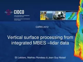
Vertical surface processing from integrated MBES – lidar data

1. CARIS 2012 Vertical surface processing from integrated MBES –lidar data Eli Leblanc, Mathieu Rondeau & Jean-Guy Nistad

2. Introduction • In the last few years, CIDCO has been developing expertise in port infrastructure inspection • Current method: subjective and partial observations from divers • CIDCO method: objective, full coverage and efficient sonar-lidar 3D dataset

3. Introduction

4. Introduction • For the first time, port management bodies have a full view of the submerged part of their structures • Precious information tobetter plan maintenanceand repair

5. Introduction • 3D points cloud is not easily usable by engineers • Uncertainty on the sonar 3D dataset exceeds the clients specifications of 5 cm • Vertical surfaceprocessing is not yetsupported in CARIS HIPS

6. Introduction • 3D points cloud is not easily usable by engineers • Uncertainty on the sonar 3D dataset exceeds the clients specifications of 5 cm • Vertical surfaceprocessing is not yetsupported in CARIS HIPS

7. Introduction • 3 solutions were tested 1) Vessel file roll bias (HIPS) 2) Inverse-distance WMA filter (HIPS-Matlab) 3) XTF files rotation (Matlab-HIPS)

8. Dataset • Port of Montréal • November 2011 • 30° tilted MBES Reson Seabat 7125 • Data recorded in xtf format

9. Dataset ALMIS 350 GPS IMU LiDAR Scanner Camera Reson 7125 SV 30° starboard tilted

10. Dataset

11. 1) Vessel file roll bias • 90° roll bias applied to the vessel file during merging → HIPS • BASE surface → HIPS

12. 1) Vessel file roll bias • Original sonar data (observed depths)

13. 1) Vessel file roll bias • Step 1:90° roll bias in the vessel file

14. 1) Vessel file roll bias • Step 1:Sound velocity correction

15. 1) Vessel file roll bias • Step : Merge the line (processed depths)

16. 1) Vessel file roll bias • Step 3:Merge the line

17. 1) Vessel file roll bias • Step 4: Remove the seabed

18. 1) Vessel file roll bias • Step 5: Create a BASE surface • Swath angle, 10 cm

19. 1) Vessel file roll bias • Limits • Roll bias applied in sonar referential at each ping rather than at a fixed rotation point • Distortion • Impossible to process multiple lines

20. 1) Vessel file roll bias • Limits • Roll bias applied in sonar referential at each ping rather than at a fixed rotation point • Distortion • Impossible to process multiple lines

21. 2) Inverse-distance WMA filter • Data merging → HIPS • Filtering and surface meshing → Matlab

22. 2) Inverse-distance WMA filter • Step 1: Export merged data from HIPS and load them in Matlab

23. 2) Inverse-distance WMA filter • Step 2: Remove the seabed (depth threshold)

24. 2) Inverse-distance WMA filter • Step 2: Model the infrastructure axis and rotate around z θaxis x y

25. 2) Inverse-distance WMA filter • Inverse-distance weight moving average filter (10 cm, r = 14.14 cm)

26. 2) Inverse-distance WMA filter • Limits of the method • Costly in computation time • 4 lines = 150 m = 750 000 soundings = 30 minutes • Possible memory problems for larger datasets • No shadow effects or texture

27. 3) XTF files rotation • 90° rotation applied on xtf files → Matlab • Data cleaning, merging and BASE surface → HIPS

28. 3) XTF files rotation • Step 1: Extractfieldsfromxtf files • For eachswath • x-y coordinates • Pitch, roll, heave,heading • For eachsounding • Two-way travel time • Angle z (x,y) (t,θ) t θ y x

29. Step 2: Model the infrastructure axis and rotate around z 3) XTF files rotation θaxis θ'heading θheading x y

30. 3) XTF files rotation z • Step 3: Compute range (x,y)sonar heave R y θ x (t,θ)sounding

31. 3) XTF files rotation z • Step 4: Project (x,y)sonar across swath (x,y)sonar heave R y θ x (x,y,z)sounding

32. 3) XTF files rotation z z • Step 5: Rotate around x (90°) y y x x 90°

33. 3) XTF files rotation z z • Step 5: Rotate around x (90°) y y x x 90°

34. 3) XTF files rotation z z • Step 5: Rotate around x (90°) y y x x 90°

35. θ θ' 3) XTF files rotation z • Step 6: Edit θ y x

36. 3) XTF files rotation • Step 7: Edit navigation - (x,y)sonar • x coordinates → infrastructure axis x' y'

37. 3) XTF files rotation • Step 7: Edit navigation - (x,y)sonar • y coordinates y x x 90° z z y

38. θ θ' (x,y,z)’sounding R 3) XTF files rotation z • Step 7: Edit navigation - (x,y)sonar • y coordinates (x,y)’sonar y x

39. 3) XTF files rotation • Step 8: Edit attitude angles (Pitch) • x-z plane • x to horizontal axis z z θpitch x y y x

40. 3) XTF files rotation • Step 8: Edit attitude angles (Pitch) • x-z plane • x to horizontal axis z z θpitch x x y y 90°

41. θ’heading 3) XTF files rotation • Step 8: Edit attitude angles (Pitch) • x-z plane • x to horizontal axis z y x x z y θpitch

42. 3) XTF files rotation • Step 8: Edit attitude angles (Heading) • x-y plane • y to horizontal axis y y θheading x x z z

43. 3) XTF files rotation • Step 8: Edit attitude angles (Heading) • x-y plane • y to horizontal axis y y θheading x x z z 90°

44. 3) XTF files rotation • Step 8: Edit attitude angles (Heading) • x-y plane • y to horizontal axis z y θheading θ'pitch x x y z

45. 3) XTF files rotation • Step 8: Edit attitude angles (roll) • y-z plane • z to vertical axis z z θroll y y x x

46. 3) XTF files rotation • Step 8: Edit attitude angles (roll) • y-z plane • z to vertical axis z z θ'roll θroll y y x x 90°

47. 3) XTF files rotation • Step 9: Edit fields to create new xtf files • For each swath • x-y coordinates • Pitch, heave, heading • For each sounding • Beam angle

48. 3) XTF files rotation • Step 10: Createa BASE surface in HIPS • Swath angle, 10 cm

49. 3) XTF files rotation • Limits of the method • Sound velocity cannot be corrected in HIPS • SVC in Matlab would imply correcting for attitude • TPU would have to be investigated to use CUBE

50. Discussion • Comparison of methods