Introduction to the Simplex Algorithm Active Learning – Module 3
Learn how to apply the simplex algorithm in linear programming, understand standard LP problem forms, and optimize solutions. Practice time management and problem-solving skills in team exercises. Solve strategy problems and readiness assessments.

Introduction to the Simplex Algorithm Active Learning – Module 3
E N D
Presentation Transcript
Introduction to the Simplex AlgorithmActive Learning – Module 3 J. René Villalobos and Gary L. Hogg Arizona State University Paul M. Griffin Georgia Institute of Technology
Background Material • Almost any introductory Operations Research book has a chapter that covers the simplex algorithm. The students should read this chapter before coming to class. Two suggestions: • Chapter 3 of Operations Research, by Hamdy A. Taha, Prentice Hall , 7th Edition • Chapter 4 of Introduction to Operations Research by Hillier and Liberman, 7th Edition • The student also should read the self-contained module on the standard form of an LP problem. This module can be downloaded from: http://enpc2675.eas.asu.edu/lobos/iie476/stdform.doc
Lecture objectives • At the end of the lecture each student should be able to: • Express a Linear Programming problem in the standard form • Set up the simplex tableau for a standard LP problem • Find the optimal solution for an LP problem using the simplex tableau
Time Management • Introduction 3 minutes • RAT 5 minutes • Lecturing on standard problem and motivation for the Simplex Algorithm 8 minutes • Individual exercise 5 minutes • Lecturing on Simplex algorithm and tableau 20 minutes • Team Exercise 5 minutes • Wrap up 4 minutes • Total lecture time 50 minutes
Report Strategy Problem • Suppose that Team members A and C have decided to work together in their tasks. They have decided that their skills are complementary and by working together in both of the tasks assigned to them they can do a better job than if they work independently. A has very good writing speed, he can write 4 pages per hour but his rate of grammatical errors is very high (3 errors per page). On the other hand, C is slower (2.5 pages per hour) but his error rate is very low (1 error per page). They want to write a report that will earn them the highest grade. They have discovered that the grade given by the professor is very much influenced by the number of pages of the written assignments (the more pages the higher the grade assigned). However, they have also discovered that for every five errors in grammar, he deducts the equivalent of one written page, and also that the maximum number of mistakes the instructor will tolerate in an assignment is 80. Help this team of students to determine the best strategy (you need to define the meaning of this) given the total time constraint available to work in the project. The total time allocated to both of them is 8 hours. Also because of previous commitments C cannot work more than 6 hours in the project
Team exercise Readiness Assessment test(5 minutes) • For the report strategy problem: • You have found graphically the optimal solution. Based on that solution do the following exercise. • You are given the alternative of increasing the number of errors allowed to 90 or to increase the number of total number of hours allowed to work in the project to 9 (for both team members). What option would you choose? Explain. • At the end of the exercise each team should turn in the individual and team solutions in a single package for grading • The instructor may select a member of the team to present the their solution to the rest of the class
x c 40 30 20 10 x A 10 20 30 Solution • From last lecture the LP formulation of the problem is: Maximize z = 1.6XA + 2.0XC Subject to: 12 XA + 2.5XC 80 XA + XC 8 XC 6 XA, XC 0 XA = 6.31, XC =1.68,Z= 13.456 XA = 2, XC =6,Z= 15.2 How many corner point solutions?
Solution (cont.) To answer the second question if we increase the number of errors to 90 the first constraint would become: 12 XA + 2.5XC 90 Then to find the point where the two constraints intersect we would have to solve the set of equations 12 XA + 2.5XC =90 XA + XC = 8 Which would give us: XA=7.368 XC = 0.6315. The objective function evaluated at this point would be 13.05 (No increase of the optimal solution non-binding constraint) Doing the same with the other constraint we get 12 XA + 2.5XC =80 XA + XC = 9 Which would give us :XA=6.05 XC = 2.94. The objective function evaluated at this point would be 15.57Increase of the optimal solutionBinding constraint We choose to increase the number of hours instead of the number of errors allowed
x c 40 30 20 10 x A 10 20 30 Solution (cont.) What is the new value of the optimal solution? The constraints that determine the value of optimal solution are called “Binding Constraints” Changes in the right hand side (RHS) of the binding constraints result in changes of the value of the optimal solution In this example the constraint affected is a non-binding constraint XA = 2, XC =6,Z= 15.2 XA = 7.368 , XC = 0.6315,Z= 13.05
Solution (cont.) • Notice that by increasing (or decreasing) the availability of a scarce resource (hours or total number of errors allowed) the straight line (representing the constraint) moves in parallel to the original one (but note that the slope does not change) • Also note that the “total-errors” constraint is a non-binding constraint. That is, it does not impact the current optimal solution. (at what point is this no longer true?)
Finding the Optimal Solution • Unfortunately we can get the graphical solution of the LP problem only for problems with 2 and 3 decision variables • Therefore we need to find an alternative method to get the optimal solution of LP problems • Some observations: • We know that the optimal solution must be in a corner point (why?) • We also know that a corner point is defined by the intersection of two constraints (for the 2 decision variable case we solve a different subset of two linear equations for each corner point). What about when we have three or more decision variables? Can you identify all the corner points? • So what we could do is solve the subsets of linear equations corresponding to all the corner points. Then we evaluate the objective function at those corner points and the one yielding the best objective value is our optimal solution. • However, since there is a large number of corner points (how many?) this is impractical. We need a smart way to search for the optimal solution. This is what the the simplex algorithm does for us.
Introduction to the Simplex Method • Simplex Method .- An algebraic, iterative method to solve linear programming problems. • The simplex method identifies an initial basic solution (Corner point) and then systematically moves to an adjacent basic solution, which improves the value of the objective function. Eventually, this new basic solution will be the optimal solution. • The simplex method requires that the problem is expressed as a standard LP problem (see module on Standard Form). This implies that all the constraints are expressed as equations by adding slack or surplus variables. • The method uses Gaussian elimination (sweep out method) to solve the linear simultaneous equations generated in the process.
Example of use of Slack and Surplus Variables 6 X1 + 3X2 10 (1) 3 X1 + X2 = 7 (2) 7 X1 + 4X2 + X3 10 (3) • Since (1) and (3) are inequalities we need to add a slack (1) and subtract a surplus variable (3) accordingly. Then the inequalities can be expressed as equations of the form: 6 X1 + 3X2 + S1 = 10 (1’) 3 X1 + X2 = 7 (2’) 7 X1 + 4X2 + X3 – S3 =10 (3’), Where S1 is a slack variable and S3 is a surplus variable. What is the physical meaning of these variables?
Example Reddy Mikks Problem Reddy Mikks Problem with slack variables Maximize z = 3XE + 2XI + 0S1 + 0S2 + 0S3+ 0S4 Subject to: XE + 2XI + S1 = 6 (1) 2XE + XI + S2 = 8 (2) -XE + XI + S3 = 1 (3) XI + S4= 2 (4) XE , XI,, S1,, S2,, S3,, S4 0 Original Reddy Mikks Problem Maximize z = 3XE + 2XI Subject to: XE + 2XI 6 (1) 2XE + XI 8 (2) -XE + XI 1 (3) XI 2 (4) XE , XI,, 0
Example Inspection Problem Inspection Problem with slack and surplus variables Minimize Z = 40 X1 + 36X2+ 0S1 + 0S2 + 0S3 Subject to: 5X1 + 3X2 - S1 = 45 X1 + S2 = 8 X2 + S3 = 10 X1, X2 S1,, S2,, S3, 0 Original Inspection Problem Minimize Z = 40 X1 + 36X2 Subject to: 5X1 + 3X2 45 X1 8 X2 10 X1, X2 0
Individual Exercise (3 min) • For the report strategy problem add the following constraint XA + XC 2 • For the resulting LP Model introduce the appropriate slack and surplus variables in the constraints and objective function • Find the maximum number of basic solutions and identify the subset of Basic Feasible Solutions on the graph.
Solution Maximize z = 1.6XA + 2.0XC + 0S1+ 0S2+ 0S3+ 0S4 Subject to: 12 XA + 2.5XC + S1 =80 XA + XC + S2 = 8 XC + S3 = 6 XA + XC – S4 = 2 XA, XC , S1 , S2 , S3 , S4 0 XA = 2, XC =6 x c XA = 6.31, XC =1.68 10 XA = 0, XC =2 x A 10
Standard Form Linear Programming • We define the standard form of a linear programming problem as: • One whose objective function is maximization • One whose constraints are expressed as equations and whose right hand side is non-negative (after the introduction of slack and surplus variables) • One in which all the decision variables are non-negative
Terminology • A solution is any specification of values for the decision variables. • A feasible Solution is a solution for which all the constraints are satisfied. • The feasible region is the set of all feasible solutions. • An Optimal Solution is a feasible solution that has the most favorable value of the objective function. • A Corner-Point Solutioncorresponds to a solution of the subset of equations corresponding to the constraints meeting at that corner point (vertex) • A Corner-point feasible (CPF) solution is a solution that lies at a corner of the feasible region . • A Basic Solution is a corner-point solution • A Basic Feasible Solution is a CPF solution for which all the variables are greater than or equal to zero.
Conceptual Outline of the Steps of the Simplex Algorithm • Step 0: Using the standard form determine a starting basic feasible solution by setting n-m non-basic variables to zero. • Step 1: Select an entering variable from among the current non-basic variables, which gives the largest per-unit improvement in the value of the objective function. If none exists stop; the current basic solution is optimal. Otherwise go to Step 2. • Step 2: Select a leaving variable from among the current basic variables that must now be set to zero (become non-basic) when the entering variable becomes basic. • Step 3: Determine the new basic solution by making the entering variable, basic; and the leaving variable, non-basic, and return to Step 1.
Simplex Method in Tableau Format • The tableau format allows us to represent the problem compactly and more easily solve it. • We merely record the coefficients of the problem only. • In order to use the Tableau Method we need to do three things first: • Represent the LP problem in standard form • Represent the objective function as an equation where z is the value of the objective function. • Determine the initial basic solution
Setting up the Reddy-Mikks Problem • For Instance the Reddy-Mikks Problem: Maximize z = 3XE+ 2XI Subject to: XE+ 2XI 6 (1) 2XE+ XI 8 (2) -XE+ XI 1 (3) XI 2 (4) XE, XI, 0 • Is expressed as: z - 3XE- 2XI - 0S1 - 0S2 - 0S3- 0S4 Subject to: XE+ 2XI + S1 = 6 (1) 2XE+ XI + S2 = 8 (2) -XE+ XI + S3 = 1 (3) XI + S4= 2 (4) XE, XI,, S1,, S2,, S3,, S4 0 Maximization is implied by the (+1)z since it is the objective function of the standard form. Because they provide an immediate basic feasible solution we choose the slack variables as the initial basic variables
Header Objective Function Constraints Simplex Tableau • The tabular form of the simplex method uses a simplex tableau to display the system of equations yielding the current basic feasible solution. • There are different ways to design the tableau a common design is as follows Initial Tableau for the R-M problem (Iteration 0)
Steps of the Simplex Algorithm • Step 0: Optimality test: the current basic feasible solution is optimal if every coefficient in row 0 of the tableau is non-negative. If it is, stop; if not perform an additional iteration. • Step 1: Determine the entering variable by selecting the variable having the most negative coefficient in row 0. The corresponding column is called the pivotcolumn. • Step 2: Determine the leaving variable by applying the minimum ratio test: • Pick out each coefficient in the pivot column having a positive value. • Divide the right hand of each row by each of these positive coefficients. • Determine the smallest of these ratios • The basic variable for the row corresponding to the smallest ratio is the leaving variable. Replace this variable with the entering variable in the next tableau. • The row with the smallest ratio is called the pivot row. The number in the intersection of the pivot column and row is the pivot element. • Step 3: Solve for the new BFS by using elementary row operations.
6/1 8/2 Leaving Variable: Smallest ratio obtained by dividing the RHS of each row by the positive coefficients of the entering variable (Column) Entering Variable: Select the variable with the most negative coefficient in the objective function Iteration 0 (Steps 0,1,2) Pivot Element
Iteration 0 (Step 3) • To get the new BFS we perform the following steps • Divide the pivot row by the pivot element and call it the “new pivot row”. Copy the result in the tableau for the next iteration • For every row of the current tableau (excluding the pivot row) subtract the product of its pivot-column coefficient times the new pivot row. Copy the result in the corresponding row of the next-iteration tableau. Make sure to properly identify the new basic variable. • M-R Example: New pivot 1:
M-R Example: New Row 1 Original Equation 1 (-1) Minus (1) times new pivot row New Equation 1 Resulting Tableau (Partial)
Team exercise (5 minutes) • Perform the operations needed to get the resulting equation 0 • The instructor might select a member of the team to present the team’s solution to the rest of the class
Result of Exercise Original Equation 0 Minus (-3) times new pivot row New Equation 0
2/1.5 4/0.5 5/1.5 2/1.0 Entering Variable: Select the variable with the most negative coefficient in the objective function Iteration 1 Leaving Variable: Smallest ratio obtained by dividing the RHS of each row by the positive coefficients of the entering variable (Column)
Iteration 2 Since all the coefficients in the objective function are positive we stop: We have found the optimal Solution
Using the Simplex procedure for Minimization problems • A minimization problem can be converted to a maximization problem just by multiplying the objective function by (-1). • Once this is done the problem is solved exactly the same as the maximization problem • Example: Minimize z = x1- 3x2 –2x3 Subject to: 3x1 - x2 + 2x3 7 -2x1 + 4x2 + 2x3 12 -4x1 + 3x2 + 8x3 10 x1, x2 0 Maximize (-z) = -x1+ 3x2 + 2x3 Subject to: 3x1 - x2 + 2x3 7 -2x1 + 4x2 + 2x3 12 -4x1 + 3x2 + 8x3 10 x1, x2 0 Max. –z + x1 - 3x2 –2x3 = 0 Subject to: 3x1 - x2 + 2x3 + S1 = 7 -2x1 + 4x2 + 2x3+ S2 = 12 -4x1 + 3x2 + 8x3 + S3 = 10 x1, x2, S1 , S2, S3, 0
Team Exercise (5 minutes) • Setup the tableau and perform one iteration of the Simplex Algorithm • Answer the following question: How would you evaluate the efficiency of the simplex algorithm? • The instructor may select a member of the team to present the team’s solution to the rest of the class
Solution • Efficiency of the simplex algorithm • One way to assess the efficiency of the simplex algorithm is to count the number of iteration needed to arrive to the optimal solution and to compare this against the total number of corner point solutions given by the formula: • (n) = number of variables, (m) = number of equations
Assignment • Setup the tableau and perform the first iteration for the report strategy problem • Using the software provided with your textbook solve the Reddy-Mikks and the report strategy problem
Corner Point Solution • Previously we learned that a corner point solution corresponds to a solution of the subset of equations corresponding to the constraints meeting at that corner point (vertex) • Thus if we have m constraints and n dimensions we use only n equations to find the corner point solution.