Understanding the Simplex Method for Linear Programming
110 likes | 251 Vues
This document provides a comprehensive overview of the Simplex Method, an algorithm for solving linear programming (LP) problems developed by George Dantzig in 1947. It details the process of finding optimal solutions by examining feasible corner point solutions through iterative algorithms. The text explains the conversion of functional inequality constraints to equality constraints using slack variables, the construction of the simplex tableau, and the steps for performing iterations and optimality tests. Key aspects like sensitivity analysis, duality theory, and applications in various programming frameworks are also discussed.

Understanding the Simplex Method for Linear Programming
E N D
Presentation Transcript
Public Policy ModelingSimplex MethodFriday, September 26, 2014 Hun Myoung Park, Ph.D. Public Management & Policy Analysis ProgramGraduate School of International Relations
Simplex Method • Algorithm to solving LP problems. • Developed by George Dantzig in 1947 • Search for optimal solution by examining corner point feasible solutions (corner solutions) • Iteration algorithm keeps searching until finding the optimal solution. • Efficient algorithm to reach the optimal solution by focusing on corner solutions • Informative to provide valuable information such as shadow price (sensitivity analysis)
Augmented Form 1 • Convert the functional inequality constraints to equivalent equality constraints by introducing slack variables
Augmented Form 2 • The original form has been augmented by some supplementary variables (slack variables) • Augmented solution is a solution for the original variables that has been augmented by the corresponding values of the slack variables. • Basic solution is an augmented corner-point solution and • Basic feasible (BF) solution is an augmented corner point feasible (CPF) solution
Simplex Method 1 • Tabular form is often used • Use augmented form with equality constraints • Construct a simplex tableau • A simplex tableau summarizes coefficients in the middle and result values on the right side • Objective function Z always appears on the top. • The Z value appear on the right side column • Right side contains the (initial) basic feasible solution. • See Excel Worksheet for an example.
Simplex Method 2 • An example of an Initial Simplex Tableau
Simplex Method 4 • InitializationOptimality TestIteration Optimality test… Initialization: construct the initial simplex tableau • Decision variables remain nonbasic variables (set equal to zero) • Slack variables become basic variables that appear on the left. • Optimality test: if and only if every coefficient in row for Z is nonnegative (>=0) current BF solution is optimal. Otherwise, go to an iteration.
Simplex Method 5 • Iteration 1: determine the entering basic variable (to be basic variables in the next iteration) with the negative coefficient having the largest absolute value. The column for such variable is called pivot column. • Iteration 2: determine the leaving basic variable (to be nonbasic variables in the next iteration) using minimum ratio test. • See pp.103-107 of Hillier & Lieberman (2010)
Simplex Method 6 • Minimum ratio test: • Pick out each positive (>0) coefficient in the pivot column • Divide right side values by positive coefficients • Identify the row having the smallest ratio • The row (basic variable) is leaving basic variable and is called pivot row. • The value in pivot column and row is pivot number. • Minimum ratio test determine which basic variable drops to zero first as the entering basic variable is increased.
Simplex Method 7 • Iteration 3: solve for the new basic feasible solution by Gauss-Jordan method of elimination • Divide the pivot row by the pivot number • Identify a row other than pivot row that has nonzero coefficient in the pivot column • Multiply the pivot row by the coefficient and then subtract the pivot row from the row of interest. • Repeat it to other row having nonzero coefficient in the pivot column • Optimality Test to see if every coefficients in row Z are nonnegative.
Further Directions • Duality Theory: primal versus dual problem • Transportation and Assignment • Integer (Binary) Programming • Goal Programming
