DNA Forensics
Explore the use of recombinant DNA technology in forensic investigations, focusing on human identification, kinship analysis, and statistical assessments of DNA evidence. Learn from experts in the field about current paradigms, challenges, and probabilistic calculations. Gain insights into the history, markers, scenarios, and statistical logic of DNA forensics.

DNA Forensics
E N D
Presentation Transcript
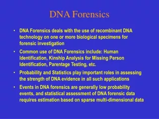
DNA Forensics • DNA Forensics deals with the use of recombinant DNA technology on one or more biological specimens for forensic investigation • Common use of DNA Forensics include: Human Identification, Kinship Analysis for Missing Person Identification, Parentage Testing, etc. • Probability and Statistics play important roles in assessing the strength of DNA evidence in all such applications • Events in DNA forensics are generally low probability events, and statistical assessment of DNA forensic data requires estimation based on sparse multi-dimensional data
Brief Introduction of the DNA Forensics Session of the Symposium • Four talks will address some of the major Statistical/Probabilistic issues of DNA Forensics • Current paradigm of the topic will be the focus of the first talk (R. Chakraborty) • B. Budowle will address challenges to such paradigm, when DNA quantity is low, and for identification of source of microbial agents in forensic samples • T. Wang will introduce the need of pedigree-based probabilistic calculations for missing person identification • A. Eisenberg will discuss possible statistical formulations applicable for newer technologies that being (or, about to be) implemented in the field • All four speakers are major players in DNA Forensics in the country; contributed significantly in the development of DNA Forensics; and together, have over 75 years of experience working in the subject
Statistical and Probabilistic Issues in DNA Forensics: Current Paradigms Ranajit Chakraborty, PhD Robert A. Kehoe Professor and Director Center for Genome Information Department of Environmental Health University of Cincinnati College of Medicine Cincinnati, OH 45267, USA Tel. (513) 558-4925/3757; Fax (513) 558-4505 e-mail: ranajit.chakraborty@uc.edu (Presentation at the University of Cincinnati Symposium on Probability Theory and Applications on March 21, 2009)
Overview of the Talk • Brief History of DNA Forensics • Currently used DNA Markers in Forensics • Three Generic Forensic Scenarios • Examples of DNA Evidence Data • Frequency, Likelihood, and Bayesian Logic of DNA Statistics • Population Substructure and Its Effect on DNA Statistics • Lineage Markers (mtDNA and Y-STR haplotypes) • Match and Partial Match in Databases
Brief History of DNA Forensics • 1980 – Ray White described the first hypervariable RFLP marker • 1985 – Alec Jeffreys discovered multilocus VNTR probes (the term “DNA Fingerprinting” coined) • 1985 – First paper on PCR published • 1988 – In US, FBI started DNA forensic casework • 1991 – First STR paper published • 1992 – NRC-I Report Issued • 1994 –CODIS STR Loci Characterized • 1995 – FSS started UK DNA Database • 1996 – NRC-II Report Issued; mtDNA introduced in Forensics • 1997 – 13 CODIS STR Loci Validated for Forensic Use; Y-STRs described for forensic investigation purposes • 1998 – FBI launched CODIS Database • 2000 – RFLP Technology replaced by Multiplex STR Technology • 2002 – FBI mtDNA Population Database published; Y-STR 20plex published • 2002 – SNPs have been proposed as supplementary markers • 2004 – Large sizes of “offenders’ data bases” opened issues of coincidental full/partial matches • 2007 – Familial search through partial match occurrences in databases
Advantages of Use of STR Loci in DNA Forensics CSF1PO D7S820 TPOX D8S1179 THO1 D13S317 FGA D16S539 VWA D18S51 D3S1358 D21S11 D5S818 Penta D Penta E • PCR Based • Low quantity DNA • Degraded DNA • Amenable to automation • Non-isotopic • Rapid typing • Discrete alleles • Abundant in genome • Highly informative (satisfied by the CODIS STRs)
15 CODIS STR Loci with Chromosomal Positions TPOX D3S1358 TH01 D8S1179 D5S818 VWA FGA D7S820 CSF1PO AMEL Penta E D13S317 AMEL D16S539 D18S51 D21S11, Penta D
Three Types of DNA Forensic Issues • Transfer Evidence: DNA profile of the evidence sample providing indications of it being of a single source origin • Mixture of DNA: Evidence sample’s DNA profile suggests it being a mixture of DNA from multiple (more than one) individuals • Kinship Determination: Evidence sample’s DNA compared with that of one or more reference profiles is to be used to determine the validity of stated biological relatedness among individuals
DNA Mixture Analysis (amelogenin, D8S1179, D21S11, D18S51)
Y-Chromosomal Genes Lahn, Pearson & Jegalian 2001
Three Types of Conclusions • Exclusion • Match, or Inclusion • Inconclusive
Statistical Assessment of DNA Evidence • Needed most frequently in the inclusionary events • (Apparent) exclusionary cases may also be sometimes subjected to statistical assessment, particularly for kinship determination because of genetic events such as mutation, recombination, etc. • Loci providing inconclusive results are often excluded from statistical considerations • Even if one or more loci show inconclusive results, inclusionary observations of the other typed loci can be subjected to statistical assessment
Approaches for Statistical Assessment of DNA Evidence Frequentist Approach: indicating the coincidental chance of the event observed Likelihood Approach:indicating relative support of the event observed under two contrasting (mutually exclusive) stipulations regarding the source of the evidence sample Bayesian Approach: providing a posterior probability regarding the source, when data in hand is considered with a prior probability of the knowledge of the source (later is not generally provided by the DNA profiles being considered for statistical assessment)
Frequentist Approach of Statistical Assessment for Transfer Evidence When the evidence sample DNA profile matches that of the reference sample, one or more of the following questions are answered: • How often a random person would provide such a DNA match? Equivalently, what is the expected frequency of the profile observed in the evidence sample? – also called Random Match Probability, complement of which is the Exclusion Probability • What is the expected frequency of the profile seen in the evidence sample, given that it is observed in another person (namely in the reference sample) – also called Conditional Match Probability • What would be the expected frequency of the profile seen in the evidence sample in a relative (of specified kinship) of the reference individual, given the DNA match of the reference and evidence samples – also called the Match Probability in Relatives
Frequentist Approach of Statistical Assessment for DNA Mixture When the evidence mixture DNA profile fails to exclude a reference sample as a part contributor, and more commonly a set of reference samples together explains all alleles seen in the mixture, one or more of the following questions are answered: • How often a random person would be excluded as a part contributor of the mixture sample? – also called Exclusion Probability, the complement of which is the inclusion probability, giving the expected chance of Coincidental Inclusion (Note: This answer is based on the data on the evidence sample alone, without any consideration of the profiles of the reference samples) • With a stipulation on the number of contributors, how often a random person’s DNA, mixed with that of one or more of the reference persons, would provide a mixture profile as seen in the evidence sample, given that the reference persons are also part contributors of the DNA mixture (Note: This answer considers data on the profiles of evidence sample as well as those of the reference samples stipulated to be part contributors)
Kinship Assessment – Frequentist Approach When comparisons of evidence and reference samples fail to exclude a stated relationship of the evidence sample with the reference individual(s), the frequency based question is of the form: • What is the chance of excluding the stated relationship? – called the Exclusion Probability (PE), this is generally answered conditioned on the profiles of the reference samples and stated relationship Note: Average exclusion probability can also be computed disregarding the profiles examined, which rationalizes the choice of loci to be typed for validating the stated relationship
Concept of Likelihood A Likelihood represents the support of a given hypothesis (of vale of a parameter) provided by the observations in the data, written as Likelihood = Prob. (Data | Hypothesis). Technically, likelihood is mathematically identical to the probability of the data given the hypothesis, but interpreted as a function of the hypothesis (or, parameter values specified by the hypothesis) for the observationsin the data.
Likelihood Ratio With two (mutually exclusive) hypotheses, say H1 and H2, the likelihood ratio (LR) is the ratio of probabilities of observing the same data under H1 and H2 , giving LR = Prob. (Data | H1) / Prob. (Data | H2). Meaning of LR: LR < 1: Data less well supported by H1, compared with H2 LR = 1: Data equally well supported by H1 and H2 LR > 1: Data better supported by H1, compared with H2
LR in Transfer Evidence Background Data: DNA profile of evidence sample (E) matches that of the suspect (S); i.e., E = S Contrasting Scenarios of Source (Hypotheses): Hp: DNA in the evidence sample came from the suspect Hd: DNA in the evidence came from someone other than the suspect, but it coincidentally matches the DNA profile of the suspect.
LR in Transfer Evidence Computation LR = Pr. (Data |Hp) / Pr. (Data | Hd) = Pr. (E = S |Hp) / Pr. (E = S | Hd) = 1 / Pr. (coincidental match) Thus, LR in this case is simply the inverse (reciprocal) of the relative frequency of the DNA profile of the evidence sample in the population, given that it is the same as of the suspect
LR in Transfer Evidence Variation Since LR can be defined for any two mutually exclusive hypotheses, one may also consider the alternative hypothesis as: Hr: A relative of the suspect is the source of evidence DNA In this case, the likelihood ratio, LR(r), will be LR(r) = Prob. (E=S | Hp) / Prob. (E =S | Hr) = 1/ Pr. (DNA match in the relative), which equals the reciprocal of the probability of the DNA profile found in the evidence sample in the relative of the suspect, given that the suspect has the same DNA profile
LR in DNA Mixture Background Data: The DNA evidence profile, E (a DNA mixture) has alleles which are all explained by alleles present in the suspect’s DNA profile (S) and that of a victim’s DNA profile (V) Contrasting Hypotheses: Hp: DNA in the evidence sample is the mixture of DNA of the suspect and that of the victim; (i.e., Hp: E = V + S) Hd1: Evidence DNA is a mixture of DNA from the victim and that of an unknown person (i.e., Hd1: E = V + UN) Hd2: Evidence DNA is a mixture of DNA from two unknown persons (i.e., Hd2: E = UN + UN)
LR in DNA Mixture Computation Pr. (Data | Hp: E = V + S) = 1, since data represents all alleles in the mixture are explained by alleles present in V and S, and no extra alleles are present in V and/or S. Hence under Hp: E = V + S, data observed is the only possible outcome, but Pr. (Data | Hd1: E = V + UN) = relative frequency of a random person, whose DNA, mixed with the DNA of the victim, would yield a mixture that matched the evidence sample, Pr. (Data | Hd2: E = UN + UN) = relative frequency of a pair of random persons, whose DNA mixture would match the profile seen in the evidence sample
LR in DNA Mixture Interpretation LR for Hp vs. Hd1: = 1 / Pr. (Data | Hp: E = V + UN), which becomes the reciprocal of the relative frequency of a random person, whose DNA, mixed with the DNA of the victim, would yield a mixture that matched the evidence sample Likewise, LR for Hp vs. Hd2: = 1 / Pr. (Data | Hp: E = UN + UN), which is the inverse of the relative frequency of a pair of random persons, whose DNA mixture would match the profile seen in the evidence sample
Other Considerations of Computing LR in DNA Mixture Computations of numerator and denominator of LR in mixture interpretation depend on: • Precise knowledge of the number of contributors in the DNA mixture • Assumptions regarding the biological relatedness of the unknown contributors (between themselves, or with the reference individuals) • Population origin of the contributors
Likelihood Ratio in Kinship Assessment Although the logic is similar, principles of LR formulation in kinship analysis can be simply illustrated with: • Standard paternity analysis (with DNA of mother, child, and alleged father typed for several loci), and • Kinship assessment for a pair of individuals (with genotype data from one or more loci)
Interpretation of LR in Paternity Testing • LR in paternity testing, also called PI, is the ratio of two conditional probabilities • It contrasts the chance of observing the specific trio of genotypes (GC, GM, and GAF) given that AF = BF, as opposed to AF ≠ BF • PI (or LR) can be computed even when M and AF, or AF and BF, are biologically related • PI can be computed for apparent exclusion events as well, invoking mutation and/or recombination (generally leading to drastically reduced PI or LR for the loci where such events are observed)
LR in Standard Paternity Testing Data: Mother’s DNA profile (GM), and that of the child (GC) suggests that all obligatory alleles (i.e., the alleles that the child must have received from its biological father, BF) are present in the DNA profile of AF (GAF) Hypotheses contrasted: • Hp: Alleged father (AF) is the biological father (BF) of the child (M is assumed to the true mother); i.e., Hp: AF = BF • Hd:Alleged father is not the biological father, but he is not excluded from paternity (i.e., Hd: AF ≠ BF)
SAMPLING THEORY OF ALLELE FREQUENCIES • Under the mutation-drift balance, the probability of a sample in which copies of the alleleis observed, for any set of is given by • Where • freq. of allele in the population, • andG(.) is the Gamma function, in which is the coefficient of coancestry (equivalent to Fstor Gst, the coefficient of gene differentiation between subpopulations within the population)
Match Probability - Formulae under HWE with substructure adjustment unconditional conditional Homozygote (AiAi ) pi2 pi2 +θpi (1-pi) [pi (1-θ)+2θ] [pi (1-θ)+3θ] (1+θ) (1+2θ) Heterozygote (AiAj ) 2pipj 2pipj (1-θ) 2[pi (1-θ)+θ] [pj (1-θ)+θ] (1+θ) (1+2θ)
CONDITIONAL MATCH PROBABILITY • Where pi, pj are frequencies of alleles Ai and Aj , and • = coefficient of co-ancestry ( Fst/Gst) representing • extent of population substructure effect • (Balding and Nichols, 1994)
Match Probability - examples under HWE with substructure adjustment (θ=.01) unconditional conditional D3S1358 (14, 18) vWA (14, 16) FGA (23, 25) D8S1179 (12, 14) D21S11 (29, 30) D18S51 (13, 17) D5S818 (12, 12) D13S317 ( 9, 11) D7S820 (10, 10) 0.0457 0.0457 0.0495 0.0411 0.0411 0.0451 0.0218 0.0218 0.0253 0.0586 0.0586 0.0626 0.0840 0.0840 0.0881 0.0381 0.0381 0.0418 0.1252 0.1275 0.1367 0.0488 0.0488 0.0542 0.0844 0.0865 0.0949 Cumulative 3.9610-12 4.1310-12 9.1510-12 Upper bound of 95% C.I. 1.0210-11 1.0510-11 2.1710-11
Paternity Testing – Frequentist Approach Example In a standard paternity testing case, with mother’s genotype being A1A1, and the child’s A1A2, an alleged father whose genotype does not contain the A2allele would be excluded, giving where is any allele other than the allele A2. This computation assumes that no mutation occurred during the transmission of alleles across generations. Note: Average exclusion probability can also be computed disregarding the profiles examined, which rationalizes the choice of loci to be typed for validating the stated relationship
LR for Kinship of a Pair of Individuals Data: DNA profile (GX) of one individual X, compared with that (GY) of another individual Y is considered to assess the accuracy of a specified stated biological relationship between X and Y Hypotheses contrasted: • Hp: X and Y are biologically related (i.e., the stated relationship is correct) • Hd:X and Y are biologically not related Note: Comparison between two stated relationships may also be tested
IBD Probabilities – ITO Method Two individuals of genotypes GX and GY can share: • Both alleles IBD (called scenario I), • Only one allele from each is IBD (scenario T), • None of their alleles are IBD (scenario O). Their probabilities are denoted by Φ2, Φ1, and Φ0, respectively, and for any biological relatedness 0 Φ2,Φ1,Φ0 1, Φ2 + Φ1 + Φ0 = 1, and 4 Φ0Φ2Φ12
Kinship Analysis of a pair of Individuals : IBD Coefficients In Relatives
Conditional Probability of Gy given Gx for specific kinship of x and y • Stipulated kinship between x and y specifies the IBD probabilities 0, 1, 2 for x and y • For observed Gx and Gy : • Pr (Gy | Gx for the specified relationship) • = 0•Pr(Gy | Gx under O) + 1•Pr(Gy | Gx under T) • + 2•Pr(Gy | Gx under I) Rule: Conditional probability of Gy given Gx for a stated kinship is the weighted average of conditional probabilities of the same event under specified IBD described by the kinship
GENOTYPE PROBABILITIES FOR A PAIR OF INDIVIDUALS CONDITIONED BY IBD PROBABILITIES OF ALLELES
P(H | E) P(E | H ) P(H ) æ ö æ ö æ ö ç ÷ ç ÷ ç ÷ 1 1 1 = ´ ç ÷ ç ÷ ç ÷ P(H | E) P(E | H ) P(H ) è ø è ø è ø 2 2 2 Bayes Formula (Odds form) posterior odds = likelihood ratio x prior odds E = DNA evidence H1 = alleged father is biological father H2 = alleged father is not biological father Note: While the first factor of the RHS is computed from DNA evidence, the second factor, P(H1)/P(H2), is not necessarily a DNA-based information
Synthesis of Three Approaches of Statistical Assessment • Frequency-Approach provides the probability of the observed DNA evidence (unconditional as well as conditional) under a given stipulated hypothesis • Likelihood Ratio (LR) contrasts such probabilities for two mutually exclusive hypotheses • In Bayesian approach, with the use of prior probability, LR is transformed to obtain the relative odds of one hypothesis against another given the DNA data of the evidence (and that from known persons tested)
Synthesis of Three Approaches (Contd.) • The three approaches are built on one another, and hence, it is inaccurate to say one is wrong and the others are correct • LR, without the transformation with the use of the prior probability, may be incorrectly interpreted as the answer of the Bayesian computation, but the numerator and denominator of LR can be stated with frequentist’s interpretation to avoid the error of reverse conditioning • The prior probability of the Bayesian approach generally comes from non-DNA evidence, and hence, their assumptions are untestable from DNA data
Important Fact with An Example LR, by itself, is not a Bayesian Approach, and the prosecutor’s fallacy can be avoided by explaining the two conditional probabilities separately Example: Consider a mixture case, where victim’s profile (V) together with the defendant’s profile (S) explains all alleles in the mixture profile (E). Under Hp: E = V + S, the conditional probability of E given Hp is 1.0, but under Hd: E = V + UN, say the conditional probability of E given that the other contributor is unknown (UN) is 1 in 100,000. Instead of telling LR = 100,000, it is less confusing to say that if we were to assume that the mixture DNA came from the victim and this defendant, this is the only observation possible (certain), but if the other contributor is unknown, we have to sample 100,000 unrelated persons before finding one, whose DNA mixed with that of the victim would produce a profile matching the profile seen in the mixture DNA evidence sample.
Is the Extent of Population Substructure Uncertain for the Forensic Loci?
Inbreeding Coefficient (FST) African American Native American Asian Caucasian Hispanic -0.0012 0.0244 CSF1PO -0.0007 -0.0009 -0.0003 0.0071 0.0157 D13S317 -0.0008 0.0029 0.0047 0.0046 0.0268 D18S51 0.0001 0.0012 0.0011 0.0056 0.0371 D21S11 0.0008 0.0005 0.0013 0.0035 0.0764 D3S1358 -0.0009 -0.0009 0.0010 0.0028 0.0656 D5S818 -0.0001 0.0010 0.0010 0.0039 0.0201 D7S820 -0.0005 0.0000 0.0010
0.0282 -0.0005 0.0006 0.0021 0.0039 Inbreeding Coefficient (FST) African American Native American Caucasian Hispanic Asian 0.0125 D8S1179 0.0000 -0.0001 0.0005 0.0025 0.0168 FGA -0.0004 0.0004 0.0008 0.0029 0.0356 THO1 -0.0012 0.0015 0.0041 0.0058 0.0164 TPOX -0.0015 0.0021 0.0024 0.0100 0.0172 VWA -0.0011 0.0011 0.0029 0.0027 Average