Download
1 / 13
130 likes | 162 Vues
Explore the use of step functions in solving linear equations with discontinuous or impulsive forcing functions using Laplace Transform. Discover how translations and transformations affect functions in this mathematical study.

E N D
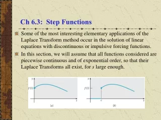
Ch 6.3: Step Functions • Some of the most interesting elementary applications of the Laplace Transform method occur in the solution of linear equations with discontinuous or impulsive forcing functions. • In this section, we will assume that all functions considered are piecewise continuous and of exponential order, so that their Laplace Transforms all exist, for s large enough.
Step Function definition • Let c 0. The unit step function, or Heaviside function, is defined by • A negative step can be represented by
Example 1 • Sketch the graph of • Solution: Recall that uc(t) is defined by • Thus and hence the graph of h(t) is a rectangular pulse.
Laplace Transform of Step Function • The Laplace Transform of uc(t) is
Translated Functions • Given a function f (t) defined for t 0, we will often want to consider the related function g(t) = uc(t) f (t - c): • Thus g represents a translation of f a distance c in the positive t direction. • In the figure below, the graph of f is given on the left, and the graph of g on the right.
Example 2 • Sketch the graph of • Solution: Recall that uc(t) is defined by • Thus and hence the graph of g(t) is a shifted parabola.
Theorem 6.3.1 • If F(s) = L{f (t)} exists for s > a 0, and if c > 0, then • Conversely, if f (t) = L-1{F(s)}, then • Thus the translation of f (t) a distance c in the positive t direction corresponds to a multiplication of F(s) by e-cs.
Theorem 6.3.1: Proof Outline • We need to show • Using the definition of the Laplace Transform, we have
Example 3 • Find the Laplace transform of • Solution: Note that • Thus
Example 4 • Find L{ f (t)}, where f is defined by • Note that f (t) = sin(t) + u/4(t) cos(t - /4), and
Example 5 • Find L-1{F(s)}, where • Solution:
Theorem 6.3.2 • If F(s) = L{f (t)} exists for s > a 0, and if c is a constant, then • Conversely, if f (t) = L-1{F(s)}, then • Thus multiplication f (t) by ect results in translating F(s) a distance c in the positive t direction, and conversely. • Proof Outline:
Example 4 • Find the inverse transform of • To solve, we first complete the square: • Since it follows that