Lenore R. Mullin James E. Raynolds
420 likes | 576 Vues
High Performance Computing from a General Formalism: Conformal Computing Techniques Illustrated with a Quantum Computing Example. Lenore R. Mullin James E. Raynolds College of College of

Lenore R. Mullin James E. Raynolds
E N D
Presentation Transcript
High Performance Computing from a General Formalism:Conformal Computing Techniques Illustrated with a Quantum Computing Example Lenore R. Mullin James E. Raynolds College of College of Computing and Information Nanoscale Science and Engineering University at Albany, State University of New York Bob Mattheyses, GE Global Research CC05 2005 14 October, 2005
Conformal Computing: streamlining computation and shedding light on physics Breakthroughs obtained by restructuring (reshaping)multidimensional arrays to suit the problem and processor/memory/FPGA hierarchy Significant advances: FFT factors of 2 to 4 speedup Bit Reversal = multi-dimensionaltranspose Fortran 95 definition is MoA definition Fundamental view: The Hypercube This talk:Conformal Computing and Density Matrices Overview
Virtual Arrays Connecting the Algorithm-Software-Hardware Boundary (ideally the Physics-Algorithm-Software-Hardware) • Array restructuring:reshape-transpose • An algebra of arrays and index calculus • MoA and Psi calculus: • Conformal Computing • Mullin-Raynolds Conjecture: • Second Fundamental Theorem of the • Psi Calculus: Reshape-Transpose • First,is thePsi Correspondence Theorem(PCT) • Mullin and Jenkins, Concurrency: Practice and Experience 9-96
Data Structure insights • The structureof density matrices • What is the structure really? • Is the matrix the ideal way of seeing a quantum algorithm? • Are there other representations more ideal? • Must we always use Permutation Matrices to permute indices? • Can we envision a quantum algorithm? • Hypercubes: L2 space
Reshape-Transpose • Array restructuring:reshape-transpose • Restructure the density matrix • Restructure to lift dimension to match processor/memory/FPGA hierarchy. • View qubits as coordinates in a hyperspace • Reshape-transpose and hypercube common themes in FFT: • bit reversal is hypercube transpose • transpose vector to define butterfly in FFT • transpose vector to define cache loop in FFT • Computer Physics Communications • Materials Research Society • Digital Signal Processing • - NO Permutation Matrices and NO Matrix Multiplication to permute indices
Example:Block Decomposition 2-dimensional Viewed as 4-dimensional
Shape operator: r returns a vector containing the lengths of each dimension Total numberof components in A is 16. Shape of A (two-dimensional): Shape of A’ (four-dimensional): Shapes are factorsof the total number of components. Factors fit the physics and factors fit the levels of processor/memory/FPGA/… Array“shapes”
“Reshape”Operator 2-dimensional • The process of“lifting”the • dimension is carried out with • the“reshape”operator A’= <2 2 2 2> r A Becomes 4-dimensional
Transposeoperatorf permutes the dimensions “Transpose”operator transpose vector
The arraysand are examples of “hypercubes” multi-dimensionalunit-cubes Often array operations simplify in the hypercube representation, e.g. bit reversal, permutations In a hypercube: all dimensions havelength 2 A hypercube allows the input vector to be viewed in thehighest dimension possible. Across dimensions every component can be related to every other component, i.e. permutations are easily made. “Hypercube”Representation
Through direct indexing, arbitrary data re-arrangements can be performed in ONE STEP This leads to exceedingly efficient computation Fundamental perspective: by viewing the data in computation in the most general way is leading to new insights into the underlying physics Notice ALSO: all the squares on the diagonal can be accessed in parallel, I.e. over the primary axis index or processor index(or cache index or whatever we are using). The punch line
From Classical to Quantum Gates Classical XOR Diagram Boolean Algebra Logic Expression: Boolean Table Reversible XOR: Controlled NOT Diagram Boolean Table Quantum NOT: Reversible Linear Algebra Computation and Gates
FromClassicaltoQuantumComputing • Basic Gates in Classical Computers • and, or, not • Basic Gates in Quantum Computers • not, controlled not, controlled- controlled not • Major Differences • ONE state versus ALL states • Boolean Algebra versus Linear Algebra • Irreversible versus Reversible • computation
x Classicalxor 2 bits in 1 out x y xor(x,y) 0 0 0 1 0 1 0 1 1 1 1 0 ( x y) + (y x) ((x=0)&(y=1)) | ((y=0)&(x=1)) y Reversiblexor 2 bits in 2 out Controlled NOT (classical implementation) cnot(x,y) x y x’ y’ 0 0 0 0 1 0 1 1 0 1 0 1 1 1 1 0 x x’ y’ y x
or Some Notation • Use matrices to denote states • The above are basis states in an abstract space (Hilbert space). • Linear Algebra to relate gate operations • Classical states use Boolean Algebra
Basis states: what are they, really? • Physical example: the states and can be realized as the spin-down and spin-upstates of a spin-1/2 particle such as an electron. • States (information) are manipulated through the application of electro-magnetic fields. • Example: application of an EM pulse can flip a state from down to up (just like in Nuclear Magnetic Resonance spectroscopy).
General state: superposition (linear combination) Some Notation (cont.)
Basis states in higher dimensions from Cartesian products of and For example A general state is a linear combination of these basis states in this 4-dimensional space: Higher Dimensions
Example: CNOT(controlled not) Y = (a|0> + b|1>)|0> = a|00> + b|10> = a|00> 0|01> b|10> 0|11> a 0 b 0 Y = = 1 0 0 0 0 1 0 0 0 0 0 1 0 0 1 0 CNOT = 1 0 0 0 0 1 0 0 0 0 0 1 0 0 1 0 a 0 0 b CNOT Y = a 0 b 0 = = a|00> + b|11>
Physical Observables • Measureable quantities calculated as averages of operators: • Wave function vs. density matrix representation
Quantum Simulators: We can’t build many qubit quantum computers YET One Method: Density Matrix Method GE Application with Lockheed Martin R. Mattheyses Quantum Density Matrix • Expresses the distribution of quantum states in an ensemble of particles prepared by a state|y> • A Density Matrix, denoted by D, is|y> <y|(the outer product) D=
Quantum Simulation • Quantum simulators: we can’t build many qubit quantum computers YET • One method: density matrix method • Computations are Gate Operations • Gate Operations are Matrix Operations • Linear Algebra • Algebra of Arrays(MoA): Algorithm and Architecture
Industrial applications • GE-Lockheed Martin Objectives • Flexible extensible simulator for quantum algorithms • Provide high performance throughput • Advanced Architectures: NEED portable, scalable designs, optimal performance. • May include multiple processors, levels of memory, FPGAs. • SGI MOATB • Cray XD1 • Exploit sparseness and structure of gate operators • Simulate systems with more than 14 qubits • In a Quantum Computer we require in excess of 231 bytes
Simulations • Why simulate? • Quantum computers are difficult to build • Usually small laboratory experiments: 4-5 qubits • Major error mechanisms can be modeled • Hardware imperfections and physical phenomena • Simulation allows observation of intermediate states • Reversible conventional gates • Use the simulator to explorequantum algorithmdevelopment fordigital and image processingapplications, e.g.FFT
Density Matrix2n X 2n to Quantum Density Hypercube2-dto2n-d • one qubit: 2 by 2 matrix • two qubits: 4 by 4 matrix • three qubits: 8 by 8 matrix • … • Goal: Create a Quantum Algorithm to perform n qubit-gate operations that is true to the physics AND computational platform.Thus, all designs are verifiable, and scalable to existing AND emerging architectures.
Density Matrix2n X 2n to Quantum Density Hypercube2-dto2n-d • View the qubits as coordinates in the Quantum • Density Hypercube • Create a permutation vector that will be used to perform a • multi-dimensional transpose on the Quantum Density • Hypercube. • The result of this transposealigns matrices on the • diagonal of the original Density Matrix • Gate is then applied, again noting the gates can be applied in parallel , i.e. the processor index is the primary axis index.
Density Matrix2n X 2n to Quantum Density Hypercube 2-d to 2n-d • Thedesign and subsequentimplementationuses the least amount of resources. • Normal formsafter MoA and Psi Analysis, • yield ageneric designindependent of platform.
Qubits, Indices, and Permutations Example: 16 by 16 Density Matrix becomes a 28 Quantum Density Hypercube Note that the design is for 2n by 2n , 0<=n, n in I+ AND any number of bits. Recall the xls file previously shown
Qubits, Indices, and Permutations • Assumptions in the Example: • Letaand bdenote which bits to gate: • xxab: bits 0 and 1 axxb: bits 0 and 3 … • bitsare numbered fromrightto left: • 1 1 1 0 is used to evaluate its decimal equivalent • ( 1 * 23 ) + ( 1 * 22 ) + ( 1 * 21 ) + ( 0 * 20 ) • indexingis numbered fromleft to right • As a vector, < 1 1 1 0 > when indexed would yield: • < 1 1 1 0 >[0] = 1 • … • < 1 1 1 0 >[3] = 0
Qubits, Indices, and Permutations • Example(cont.): From qubits to permutation vector • bits 0,2: xaxb -> 3 2 1 0 3 2 1 0bit ordering • 0 1 2 3 0 1 2 3index ordering • 0 2 13 0 2 13bit 2 is index 3 • swap bits 1 and 2 <0 2 1 3 4 6 5 7> is the transpose vector • bits 1,2: xabx -> 3 21 0 3 21 0 bit ordering • 0 12 3 0 12 3 index ordering • 0 1 32 0 1 32 swap bits 2 and 3 • 0 3 1 2 0 3 1 2swap bits 1 and 2 <0 3 1 2 4 7 5 6> is the transpose vector • bits 0,3: axxb -> <2 1 0 3 6 5 4 7> • bits 1,3: axbx -> <3 1 0 2 7 5 4 6> • bits 2,3: abxx -> <2 3 0 1 6 7 4 5>
From Permutation Vector to the Diagonal • Given: a permutation vector denoted by , the transpose vector, • permute all indices. • Apply binary transpose after reshaping(restructuring) the • density matrix into a density hypercube. • Permute all indices as defined by the transpose vector • Gated arrays are now on the diagonal.
From Permutation Vector to the Diagonal • Indices are calculated and addressed directly from the • original array stored in memory: • Algebraically the Physics • Algebraically all at once • Algebraically decomposable to present and future architectural platforms(even quantum) • Algebra remains the same throughout • the problem, • the decomposition over processor/memory/FPGA, • the mapping, • the architectural abstraction, • verifiable designs
The General ExpressionMoa and Psi Reduction Given DM s.t. rDM = < 2n 2n >, restructure to a hypercube, QDH. Let s denote the shape of QDH s.t. s= < 2nr^2 > = < 2 … 2 2 > 2n Then QDH = s r^DM Use t, the transpose vector previously defined. Perform the binary transpose: t O QDH Now, all matricesdefined by bits chosen are on the diagonal. Note: Restructuring back to DM and indexing creates no new arrays because of Psi Reduction.
The General ExpressionMoa and Psi Reduction t O QDH • This expression moves all gated coordinates to the diagonal • (after reshaping) of DM. • This expression describes the Physics in one operation. • Now Psi Reduce to normal form -> Generic Design. • forall i s.t. 0 <= i < 22n • i= g’ ( i; s ) • i = i [ t ] • @DM + g( i ; s ) • This is the Generic Normal Form
Conclusions • Moa and Psi calculus quantum algorithmfor density matrix optimizations. • Describes the physics naturally. • qubit access and gate application. • Independent of number of qubits. • Independent of density matrix size. • Describes decomposition and mapping. • Multiple processor/memory levels. • Normal form is a generic design independent of target architecture, ideally the physics directly.
The punch line • Through direct indexing, arbitrary data re-arrangements can be performed in ONE STEP • This leads to exceedingly efficient computation • Fundamental perspective: by viewing the data in computation in the most general way is leading to new insights into the underlying physics
Fundamental concepts: reshape-transpose, hypercube representation…just beginning to be explored Connections with quantum algorithms: Quantum FFT, Shor’s factoring algorithm, etc Highly efficient practical designs for today’s computers! Future Directions
We thank Robert Mattheyses from GE Global Research for introducing us to this problem. Acknowledgement