Learning HMM parameters
This document presents a comprehensive overview of Hidden Markov Models (HMMs), focusing on three critical questions: how to compute the likelihood of a sequence given an HMM, determine the most likely sequence of states, and learn an HMM from observed sequences. Key algorithms such as the Forward Algorithm, Viterbi Algorithm, and Baum-Welch Algorithm (an Expectation-Maximization approach) are discussed, along with methods for parameter estimation, including handling hidden state sequences. The document emphasizes the need for expected counts in the learning process and illustrates each step in the Baum-Welch algorithm.

Learning HMM parameters
E N D
Presentation Transcript
Learning HMM parameters Sushmita Roy BMI/CS 576 www.biostat.wisc.edu/bmi576/ sroy@biostat.wisc.edu Oct 31st, 2013
Recall the three questions in HMMs • Given a sequence of observations how likely is it an HMM to have generated it? • Forward algorithm • What is the most likely sequence of states that has generated a sequence of observations • Viterbi • How can we learn an HMM from a set of sequences? • Forward-backward or Baum-Welch (an EM algorithm)
Learning HMMs from data • Parameter estimation • If we knew the state sequence it would be easy to estimate the parameters • But we need to work with hidden state sequences • Use “expected” counts of state transitions
begin end Learning without hidden information • Learning is simple if we know the correct path for each sequence in our training set 0 2 2 4 4 5 C A G T 1 3 0 5 2 4 • Estimate parameters by counting the number of times each parameter is used across the training set
Learning without hidden information • Transition probabilities • Emission probabilities Number of transitions from k to l k,l are states Number of times b is emitted from k
begin end Learning with hidden information • if we don’t know the correct path for each sequence in our training set, consider all possible paths for the sequence ? ? ? ? 0 5 C A G T 1 3 0 5 2 4 • estimate parameters through a procedure that counts the expected number of times each parameter is used across the training set
The Baum-Welch algorithm • Also known as Forward-backward algorithm • An Expectation Maximization algorithm • Expectation: Estimate the “expected” number of times there are transitions and emissions (using current values of parameters) • Maximization: Estimate parameters given hidden variables • Hidden variables are the state transitions and emission counts
The expectation step • We need to know the probability of the ith symbol being produced by state k, given sequencex(posterior probability of state k at time t) • We also need to know the probability of ith and (i+1)th symbol being produced by state k, and lgiven sequencex • Given these we can compute our expected counts for state transitions, character emissions
Computing • We will do this in a somewhat indirect manner • First we compute the probability of the entire observed sequence with the tthsymbol being generated by state k Forward algorithm fk(t) Backward algorithm bk(t)
Computing • If we can compute • How can we get Forward step
The backward algorithm • the backward algorithm gives us , the probability of observing the rest of x, given that we’re in state kafter icharacters 0.4 0.2 A 0.4 C 0.1 G 0.2 T 0.3 A 0.2 C 0.3 G 0.3 T 0.2 0.8 0.6 0.5 1 3 begin end 0 5 A 0.4 C 0.1 G 0.1 T 0.4 A 0.1 C 0.4 G 0.4 T 0.1 0.5 0.9 0.2 2 4 0.1 0.8 C A G T
Steps of the backward algorithm • Initialization (t=T) • Recursion (t=T-1 to 1) • Termination
Computing • This is
Putting it all together • We need the expected number of times c is emitted by state k • And the expected number of times k transitions to l Training sequences
The maximization step • Estimate new emission parameters by: • Estimate new transition parameters by • Just like in the simple case but typically we’ll do some “smoothing” (e.g. add pseudocounts)
The Baum-Welch algorithm • initialize the parameters of the HMM • iterate until convergence • initialize , with pseudocounts • E-step: for each training set sequence j= 1…n • calculate values for sequence j • calculate values for sequence j • add the contribution of sequence j to , • M-step: update the HMM parameters using ,
begin end A 0.4 C 0.1 G 0.1 T 0.4 A 0.1 C 0.4 G 0.4 T 0.1 1.0 0.2 0.9 0 3 1 2 0.1 0.8 Baum-Welch algorithm example • given • the HMM with the parameters initialized as shown • the training sequences TAG, ACG • we’ll work through one iteration of Baum-Welch
Baum-Welch example (cont) • Determining the forward values for TAG • Here we compute just the values that are needed for computing successive values. • For example, no point in calculating f1(3) • In a similar way, we also compute forward values forACG
Baum-Welch example (cont) • Determining the backward values for TAG • Again, here we compute just the values that are needed • In a similar way, we also compute backward values for ACG
Baum-Welch example (cont) • determining the expected emission counts for state 1 contribution of TAG contribution of ACG pseudocount *note that the forward/backward values in these two columns differ; in each column they are computed for the sequence associated with the column
Baum-Welch example (cont) • determining the expected transition counts for state 1 (not using pseudocounts) • in a similar way, we also determine the expected emission/transition counts for state 2 Contribution of TAG Contribution of ACG
Baum-Welch example (cont) • determining probabilities for state 1
Summary • Three problems in HMMs • Probability of an observed sequence • Forward algorithm • Most likely path for an observed sequence • Viterbi • Can be used for segmentation of observed sequence • Parameter estimation • Baum-Welch • The backward algorithm is used to compute a quantity needed to estimate the posterior of a state given the entire observed sequence