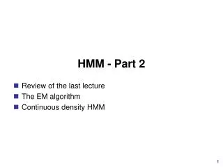
HMM - Part 2
430 likes | 701 Vues
HMM - Part 2. The EM algorithm Continuous density HMM. The EM Algorithm. EM: Expectation Maximization Why EM? Simple optimization algorithms for likelihood functions rely on the intermediate variables, called latent data For HMM , the state sequence is the latent data

HMM - Part 2
E N D
Presentation Transcript
HMM - Part 2 • The EM algorithm • Continuous density HMM
The EM Algorithm • EM: Expectation Maximization • Why EM? • Simple optimization algorithms for likelihood functions rely on the intermediate variables, called latent dataFor HMM, the state sequence is the latent data • Direct access to the data necessary to estimate the parameters is impossible or difficultFor HMM, it is almost impossible to estimate (A, B, ) without considering the state sequence • Two Major Steps : • E step: calculate expectation with respect to the latent data given the current estimate of the parameters and the observations • M step: estimate a new set of parameters according to Maximum Likelihood (ML) or Maximum A Posteriori (MAP) criteria ML vs. MAP
Expectation The EM Algorithm (cont.) • The EM algorithm is important to HMMs and many other model learning techniques • Basic idea • Assume we have and the probability that each Q=q occurred in the generation of O=o i.e., we have in fact observed a complete data pair (o,q) with frequency proportional to the probability P(O=o,Q=q|) • We then find a new that maximizes • It can be guaranteed that • EM can discover parameters of model to maximize the log-likelihood of the incomplete data, logP(O=o|), by iteratively maximizing the expectation of the log-likelihood of the complete data, logP(O=o,Q=q|)
Our goal is to maximize the log-likelihood of the observable data o generated by model , i.e., expectation We want The EM Algorithm (cont.)
If we choose so that , then the Q-function (auxiliary function) The EM Algorithm (cont.) 1. Jensen’s inequality: If f is a concave function, and X is a r.v., then E[f(X)]≤ f(E[X]) 2. log x ≤ x-1
Solution to Problem 3 - The EM Algorithm • The auxiliary function Where and can be expressed as
example wi yi wj yj wk yk Solution to Problem 3 - The EM Algorithm (cont.) • The auxiliary function can be rewritten as
Solution to Problem 3 - The EM Algorithm (cont.) • The auxiliary function is separated into three independent terms, each respectively corresponds to , , and • Maximization procedure on can be done by maximizing the individual terms separately subject to probability constraints • All these terms have the following form
Solution to Problem 3 - The EM Algorithm (cont.) • Proof: Apply Lagrange Multiplier Constraint
wi yi Solution to Problem 3 - The EM Algorithm (cont.)
wj yj Solution to Problem 3 - The EM Algorithm (cont.)
wk yk Solution to Problem 3 - The EM Algorithm (cont.)
Solution to Problem 3 - The EM Algorithm (cont.) • The new model parameter set can be expressed as:
Discrete vs. Continuous Density HMMs • Two major types of HMMs according to the observations • Discrete and finite observation: • The observations that all distinct states generate are finite in number, i.e., V={v1, v2, v3, ……, vM}, vkRL • In this case, the observation probability distribution in state j, B={bj(k)}, is defined as bj(k)=P(ot=vk|qt=j), 1kM, 1jNot :observation at time t, qt: state at time t bj(k) consists of only M probability values • Continuous and infinite observation: • The observations that all distinct states generate are infinite and continuous, i.e., V={v| vRL} • In this case, the observation probability distribution in state j, B={bj(v)}, is defined as bj(v)=f(ot=v|qt=j), 1jNot :observation at time t, qt: state at time t bj(v) is a continuous probability density function (pdf) and is often a mixture of Multivariate Gaussian (Normal) Distributions
Gaussian Distribution • A continuous random variable X is said to have a Gaussian distribution with mean μand variance σ2(σ>0) if X has a continuous pdf in the following form:
Multivariate Gaussian Distribution • If X=(X1,X2,X3,…,XL) is an L-dimensional random vector with a multivariate Gaussian distribution with mean vectorand covariance matrix, then the pdf can be expressed as • If X1,X2,X3,…,XLare independent random variables, the covariance matrix is reduced to diagonal, i.e.,
Observation vector Mean vector of the kth mixture of the jth state Covariance matrix of the kth mixture of the jth state Multivariate Mixture Gaussian Distribution • An L-dimensional random vector X=(X1,X2,X3,…,XL) is with a multivariate mixture Gaussian distribution if • In CDHMM,bj(v) is a continuous probability density function (pdf) and is often a mixture of multivariate Gaussian distributions
Observation-independent assumption Solution to Problem 3 – The Intuitive View (CDHMM) • Define a new variable t(j,k) • probability of being in state j at time t with the k-th mixture component accounting for ot
Solution to Problem 3 – The Intuitive View (CDHMM) (cont.) • Re-estimation formulae for are
Solution to Problem 3 - The EM Algorithm(CDHMM) • Express with respect to each single mixture component K: one of the possible mixture component sequence along with the state sequence Q
Solution to Problem 3 - The EM Algorithm(CDHMM) (cont.) • The auxiliary function can be written as: • Compared to the DHMM case, we need to further solve
wk yk Solution to Problem 3 - The EM Algorithm(CDHMM) (cont.) • The new model parameter set can be derived as
Solution to Problem 3 - The EM Algorithm(CDHMM) (cont.) • The new model parameter sets can be derived as
Since We want to find to maximize Solution to Problem 3 - The EM Algorithm(CDHMM) (cont.) We thus solve
HMM Topology • Speech is a time-evolving non-stationary signal • Each HMM state has the ability to capture some quasi-stationary segment in the non-stationary speech signal • A left-to-right topology is a natural candidate to model the speech signal • Each state has a state-dependent output probability distribution that can be used to interpret the observable speech signal • It is general to represent a phone using 3~5 states (English) and a syllable using 6~8 states (Mandarin Chinese)
HMM Limitations • HMMs have proved themselves to be a good model of speech variability in time and feature space simultaneously • There are a number of limitations in the conventional HMMs • The state duration follows an exponential distribution • Don’t provide adequate representation of the temporal structure of speech • First order (Markov) assumption: the state transition depends only on the previous state • Output-independent assumption: all observation frames are dependent on the state that generated them, not on neighboring observation frames • HMMs are well defined only for processes that are a function of a single independent variable, such as time or one-dimensional position • Although speech recognition remains the dominant field in which HMMs are applied, their use has been spreading steadily to other fields
ML vs. MAP • Estimation principle based on observationsO=[o1, o2, ……, oT] • The Maximum Likelihood (ML) principle:find the model parameter so that the likelihood P(O|) is maximum • for example, if={,}is the parameters of a multivariate normal distribution, andOis i.i.d. (independent, identically distributed), then the ML estimate of={,}is • The Maximum a Posteriori (MAP) principle:find the model parameter so that the likelihood P( |O) is maximum back
A Simple Example The Forward/Backward Procedure S1 S1 S1 State S2 S2 S2 1 2 3 Time o1 o2 o3
A Simple Example(cont.) q: 1 1 1 q: 1 1 2 Total 8 paths
Appendix - Matrix Calculus • Notation:
Appendix - Matrix Calculus (cont.) • Property 1: • proof
Appendix - Matrix Calculus (cont.) • Property 1 - Extension: • proof
Appendix - Matrix Calculus (cont.) • Property 2: • proof back
Appendix - Matrix Calculus (cont.) • Property 3: • proof
v u Appendix - Matrix Calculus (cont.) • Property 4: • proof back
Appendix - Matrix Calculus (cont.) • Property 5: • proof
Appendix - Matrix Calculus (cont.) • Property 6: • proof
Appendix - Matrix Calculus (cont.) • Property 7 : • proof
Appendix - Matrix Calculus (cont.) • Property 8 : • proof
Appendix - Matrix Calculus (cont.) • Property 9: • proof back