REGRESSION
Learn about linear regression for predicting one variable using another, calculation formulas, statistical inference, and residual analysis. Understand how to find the regression line using least squares principle.

REGRESSION
E N D
Presentation Transcript
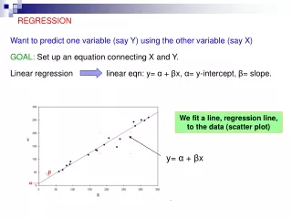
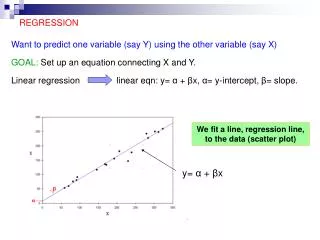
REGRESSION Want to predict one variable (say Y) using the other variable (say X) GOAL: Set up an equation connecting X and Y. Linear regression linear eqn: y= α + βx, α= y-intercept, β= slope. We fit a line, regression line, to the data (scatter plot) y= α + βx
REGRESSION LINE – understanding the coefficients Regression line: y= α + βx, α= y-intercept, β= slope Example: The study of income an savings from the last lecture. X=income, Y=savings, data in thousands $. Suppose y = - 4 + 0.14 x. Slope. Change in y per unit increase in x. For $1,000 increase in income, savings increase by 0.14($1000)=$140. Intercept. Value of y, when x=0. If one has no income, one has “-4($1000)” savings. Nonsense in this case.
REGRESSION LINE- LEAST SQUARES PRINCIPLE How to find the line of best fit to the data? Use the Least Squares Principle. Given (xi, yi). Observed value of y is yi, fitted value of y is α + βxi. Find the line, i.e. find α and β, that will minimize sum(observed –fitted)2 =sumi(yi- α - βxi) =sum(residuals)2 =sum(errors)2 Observed value = error
REGRESSION LINE - FORMULAS The least squares line y= α + βx will have slope βand intercept α such that they minimize Σi(yi- α - βxi)2. The solution to this minimization problem is and Both a and b are sample estimates of α and β. Finally, the fitted regression equation/line is NOTE: Slope of the regression line has the same sign as rXY.
EXAMPLE Income and savings. Find the regression line. Solution: Recall summary statistics: X=income, Y=savings , Σxi = 463 , Σx2i = 23533, Σyi = 27.4 , Σy2i = 120.04 ,Σxi yi =1564.4. r =0.963. Additional stats: MINITAB OUTPUT: Descriptive Statistics Variable N Mean StDev SE Mean Minimum Maximum income 10 46.30 15.26 4.83 25.00 72.00 savings 10 2.740 2.235 0.707 0.000 7.200 Then, The regression line is: savings = 0.141(income) - 3.788, in thousands of $. Range of applicability of the regression equation = about the range of the data.
INFERENCE FOR REGRESSION: t-test • The main purpose of regression is prediction of y from x. • For prediction to be meaningful, we need y to depend significantly on x. • In terms of the regression equation: y= α + βx, we need β≠0. Goal: Test hypothesis: Ho: β = 0 (y does not depend on x) Test statistic is based on the point estimate of β, Test statistic Under Ho, the test statistic has t distribution with df=n-2. For a two-sided Ha, we reject Ho if |t| > tα/2, where α is the significance level of the test. One sided alternatives, as usual.
EXAMPLE Income and savings. Does the amount of savings depend significantly on income? Use significance level 5%. Solution. Ho: β = 0(savings do not depend on income)Ha: β≠0(savings depend on income) Test statistic: and Critical number t(8)0.025=2.306. Test statistic t=10.1> 2.306, so reject Ho. Savings depend significantly on income. Estimate the p-value: 2P(T>10.1) ≈0.
(1-α)100% CONFIDENCE INTERVAL FOR β A (1-α)100% CI for β is where tα/2 is percentile from a t distribution with n-2 df. Example. Income and savings. Find 90% CI for the slope of the regression line of savings (y) on income (x). Solution. 90% CI, so α=0.1 and α/2=0.05, df=8, t0.05=1.86. 90% CI for β is:
PREDICTION Two possibilities. Given a value of x, say x* • Predict average value of y, or • Predict individual value of y for x=x*. “Average” error/residual
PREDICTION, contd. NOTE:Prediction interval for an individual value is longer than confidence interval for the mean. This is because the variability in an individual value is larger than variability in the mean. NOTE: Both intervals become longer as x* moves further from the center of the data (further from ). Example. Income and savings. Find point estimates, 90% CI for the mean savings of a family with income of $50k and PI for savings of a family with income of $50k. Solution: 90% CI or PI need t0.05 with df=8. t0.05 = 1.86. Point estimates: Average amount of savings for families with income of $50k is $3,262. For a family with income of $50k, we predict savings of $3,262.
EXAMPLE, contd. “Average” residual: 90%CI: 3.262 +/- 1.86(0.2073) = ( 2.877, 3.648). 90% PI: 3.262 +/- 1.86(0.6681) = (2.02, 4.504) longer than the CI!
CORRELATION AND REGRESSION Coefficient of determination: Say we regress Y on X: Since x changes, then changes variability in x causes variability in via regression equation. Square of the correlation coefficient r has special meaning, R2 is called coefficient of determination = fraction of variability in Y explained by variability in X via regression of y on X.
EXAMPLE Income and savings. What percent of variability in savings is explained by variability in income? Solution. The correlation coefficient was r=0.963. The coefficient of determination is r2=(0.963)2=0.927. About 92.7% of variability in savings is explained by variability in income.
REGRESSION DIAGNOSTICS: RESIDUAL ANALYSIS Regression model: Y= α+βx+ε, ε~N(0, σ) For the inference to work, we need the residuals to be approximately normal. Standard method is probability plot : use a statistical package like MINITAB. The model works well, if the normal probability plot is an approximately straight line. Example. Income and savings. The plot is approximately a straight line, so the model works well.

