Advanced Regression Techniques in Epidemiology: Applications and Interpretations
Explore advanced topics in regression analysis for epidemiology using examples like arsenic exposure and anti-epileptic drugs, including logistic, linear, and Poisson regression models. Learn model selection processes like Hosmer/Lemeshow approach and stepwise regression.

Advanced Regression Techniques in Epidemiology: Applications and Interpretations
E N D
Presentation Transcript
Regression Topics for today Readings • Jewell Chapters 12, 13, 14 & 15
Context So far in the course, we have learned how to • Quantify disease occurrence (prevalence, incidence etc) • Quantify association with an exposure (relative risk, odds ratios) and assess its significance (standard errors, confidence intervals) • Stratify for a confounding variable (Mantel-Haenszel test, Wolf or Mantel-Haenszel adjusted estimates) • Test to see if a factor influences the exposure/response association (interaction) All of this can be done with fairly simple procedures and tests. However, we’ve also been exploring how to do equivalent analyses with Poisson and Logistic regression. Today we see some additional advantages of the regression approach. Lets motivate with some examples.
Example - arsenic We’ve looked at the relative risk for the highest village (934 ppb) compared to the control group. But, we really need to characterise the whole dose response relationship. Regression allows us to do that
Example – Anti-epileptic drugs We have looked at the effect of drug exposure, adjusted for whether or not the mother smokes. But there are additional variables we would like to adjust for: • alc2: Alcohol use during pregnancy (1=yes, 0=no) • cig2: Cigarette smoking during pregnancy • sub2: Substance abuse during pregnancy • seiz: Severity of seizures (1=no seizure, 2=seizures with convulsions, 3=loss of conciousness) • mohcx2: whether mother has a small head circumference • mohtx2: whether mother has small height There is also information on the type of drug exposure • monopht: Phenytoin monotherapy • monocbz: Carbamazepine monotherapy • monopb: Penobarbital monotherapy • monooth: Other monotherapy As well as whether the mother took one drug or a combination of drugs: monostat2: Monotherapy/Polytherapy status ( 1=Polytherapy, 2=Monotherapy, 3=Seizure History,4=Controls) Regression allows us to explore some of these effects simultaneously
Type of regression models Basic concept: outcome=predicted mean+error • Linear regression – most natural when the outcome is continuous (e.g. blood pressure) • Logistic – most natural for 0/1 outcome • Poisson – most natural when outcome is count among person-years at risk, or rare disease count in population
Notes and comments • We’ve looked at some simple models where the predictors in the model are categorical. But, predictors can also be continuous. E.g. BP = β0+β1Age+error The slope (β1) tells us how much BP is predicted to increase for each 1 unit increase in age • Other models (e.g. probit – Jewell 12.3) are available, but less common • Logistic and Poisson are linear on the logit and log scales, respectively. But this induces non-linear model on mean of Y Logit(p)=-4+.1*x R command: p=exp(-4+.1*x)/(1+exp(-4+.1*x)); y=rbinom(100,1,p); plot(x,y); lines(x,p)
Example - epilepsy procgenmod descending; class drug; model one3=drug cig2 sub2 /dist=binomial; run;
How to decide what goes into a model? Hard problem - no single right answer (J15.2) Hosmer/Lemeshow approach: • Start by exploring relationship between each individual variable and the outcome • Select all the individually important variables and put into one model • Remove variables one at a time if not “significant” (look at p-values as well as likelihood ratio test) • Check if variables originally left out should go in • Consider interactions (a few limited ones) • Assess if model fits well
Example - Epilepsy Variables significant (p<.10) on their own: Drug, cig2, sub2, mohcx2, seiz,
Example continued • Dropping out the least significant, one at a time leads to model with drug, cig2 and sub2 • Note that the coefficient of mohcx2 was large, though variable not significant. Only 11 mothers had small head. It is possible (likely?) that this variable is important, but we didn’t have enough power to detect effect
Stepwise Regression Automatic variable selection procedure that will automatically sort through a dataset to find best model • Forward – start with null model and add variables one at a time • Backward – start with saturated model and remove variables one at a time • Combined – Do forward regression, but check at each step whether any variables need to be removed Can be useful, though caution needed. • Don’t overinterpret • Consider clinical/scientific relevance as well • Sometimes a useful way to start
Stepwise logistic regression in SAS proclogistic descending; class drug; model one3=drug cig2 sub2 alc2 mohtx2 mohcx2 seiz /selection=stepwise; run; Identified only drug and cig2 because 240 cases omitted because they missed one or more variables
Additional considerations for model selection • Some variables important to include, even if not “significant” • May need to decide whether to add variable as categorical or continuous or how to scale a variable (more in a moment) • Need to make sure variable is entered in a sensible way • Looking at p-values in regression model is a “quick and dirty” method. Better to look at likelihood ratio tests (see Jewell p248-9)
Dealing with continuous predictors Consider our arsenic dataset. We have two variables, concentration and agegroup. Lets run a model with both variables treated as categorical (via the class statement). Result is a HUGE regression output with each value of conc having it’s own relative risk etc
Conc as a continuous variable. Entering conc as a linear term (remove the class statement) implies a model where the log of the disease rate increases linearly with exposure, after adjusting for age. etc
Can we model age as linear too? Nice clean looking model! Is it appropriate? • Do a model comparison via LRT • Add quadratic terms to assess non-linearities
Comparing nested models via LRT Suppose model A includes model B as a special case (B is nested in A). Likelihood ratio test for modelB vs modelA is 2*(loglikA-loglikB). Compare test statistic to chi-squared distribution with df=#param(A)-#param(B).
What about non-nested models? Choose model with minimum Akaike Information Criterion: AIC =-loglikelihood/N+2*#param
Model selection can be very challenging!Especially critical for environmental risk assessment Recent Harvard Biostatistics student worked with me to apply Bayesian model averaging techniques to the arsenic data.
This is the end of my lectures! I have enjoyed being your teacher. Thank you for your kind attention and respect!

