What is a transmission line?
490 likes | 1.54k Vues
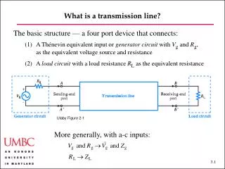
What is a transmission line?. The basic structure — a four port device that connects: (1) A Thénevin equivalent input or generator circuit with V g and R g , as the equivalent voltage source and resistance (2) A load circuit with a load resistance R L as the equivalent resistance.

What is a transmission line?
E N D
Presentation Transcript
What is a transmission line? The basic structure — a four port device that connects: (1) A Thénevin equivalent input or generator circuit with Vg and Rg, as the equivalent voltage source and resistance (2) A load circuit with a load resistance RL as the equivalent resistance Ulaby Figure 2-1 More generally, with a-c inputs:
What is a transmission line? The basic structure — a four port device that connects: (1) A Thénevin equivalent input or generator circuit with Vg and Rg, as the equivalent voltage source and resistance (2) A load circuit with a load resistance RL as the equivalent resistance Ulaby Figure 2-1 We take into account the finite transmission time from A, A′ to B, B′
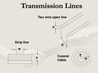
What is a transmission line? There are two basic types of transmission line: Ulaby
What is a transmission line? • A simple coaxial waveguide: • There is an electric field caused by charge separation from the inner and outer wires • There is a magnetic field that is caused by the current flow, in opposite directions, along the inner and outer conductions Ulaby Figure 2-5
Lumped Element Model • We replace the detailed physics of the transmission line with lumped circuit parameters: • R′ : The combined resistance of both conductors (ohms/meter) • L′ : The combined inductance of both conductors (henrys/meter) • G′ : The conductance of the insulating medium between conductors (siemens/meter) • C′ : The capacitance between the two conductors (farads/meter) • These parameters are all “per unit length.” Hence, we put primes. • Their values are determined by the detailed physics. • We will use this model to find a simple pair of coupled equations, The telegrapher’s equation that describes propagation through the transmission line
Lumped Element Model Transmission Line Model: Ulaby
Lumped Element Model Parameter Coaxial Two wire Parallel plane R′ L′ G′ C′ Examples of parameter determination from the physics: Ulaby Table 2-1 Slide 3.3 and the notes have definitions of a, b, d RS = surface resistance = are conductor parameters m, e, and s are insulator parameters
Microstrip Line Real transmission lines can be complex Curve fitting approximations are useful Ulaby, et al. 2010 Figure 2-10
Transmission Line Equations Our starting point is one section of the transmission line Note: We are taking a section that issmall enough so that we can assumethat the transmission through thatsection is instantaneous Ulaby Figure 2-8 Kirchoff’s voltage law: Kirchoff’s current law: (at node N + 1)
Transmission Line Equations Rearranging terms Take the limit as Δz→ 0: Telegrapher’s Equations
Transmission Line Equations • Simplification • The transmission equations become • which imply • Note: In Paul’s notation:
Transmission Line Equations The circuit diagram also simplifies The second-order wave equations become in Paul’s notation Paul Figure 6.1(c) Note change in notationfrom Ulaby L VS = source voltage RS = source resistance RL = load resistance L = total length of transmission line L L
Time-Domain Evolution • The second-order voltage equation has the general solution • V + (x) and V – (x) = two completely arbitrary functions • v = the velocity of propagation • (1) Arbitrarily shaped pulses propagate in the transmission line, both forward and backward, without dispersing! • (2) The absence of dispersion is a special feature of TEM modes, which makes direct time-domain analysis possible. Caveat: We are treating l and c as if they have no frequency dependence. This assumption is not generally true! It will often be approximately true over a limited frequency range
Time-Domain Evolution • The current is determined from the voltage— After substitution into the transmission line equations • ZC = the characteristic impedance of the transmission line • Note that since V (z, t) and I (z, t) are real, so is ZC — The characteristic impedance is purely resistive in this case. We have BUT There is no simple relationship between V(z,t) and I(z,t)!
Time-Domain Evolution Example: From Paul Quick Review Exercises 6.1 and 6.7Question: What are the per unit length capacitance and inductance of a two-wire line whose wires have a radius of 7.5 mils and a separation of 50 mils? What is the characteristic impedance and the velocity of propagation? (These dimensions are typical for ribbon cables used to interconnect components.) Answer: 7.5 mils × 2.54×10⁻⁵ m/mil = 1.91×10⁻⁴ m, 50 mils = 1.27×10⁻³ m. (d/2a) = 50.0/15.0 = 3.33, [(d /2a)2 – 1]1/2 = 3.18, ln(3.33 + 3.18) = 1.87. l = ( μ0 /π)×1.87 = 4×10⁻⁷ H/m × 1.87 = 7.46×10⁻⁷ H/m. c = (πε0/ 1.87) = (π /1.87) × 8.85×10–12 F/m = 1.49×10⁻¹¹ F/m. ZC = ( l / c)1/2 = 224 ohms. v = 1 / (7.46×10⁻⁷ H/m × 1.49 ×10⁻¹¹ F/m)1/2 = 3.00 × 10⁸ m/s. The velocity equals the speed of light in the vacuum. NOTE: Paul uses a different notation for d and ad → s, a → rw
Time-Domain Evolution We now consider the behavior at the load From Ohm’s Law: V(L,t) / I(L,t) = RL From the telegrapher’s equations: V+(t – T ) / I+(t – T ) = ZC Unless RL = ZC, there must be reflected waves! = one-way time delay L VS = source voltage RS = source resistance RL = load resistance L = total length of transmission line L L
Time-Domain Evolution We now consider the behavior at the load From Ohm’s Law: V(L,t) / I(L,t) = RL From the telegrapher’s equations: V+(t – T ) / I+(t – T ) = ZC Unless RL = ZC, there must be reflected waves! When RL = ZC, we say that the line is impedance matched = one-way time delay The concept of impedance matching is one of the most important in this course. Impedance matching is never perfect, giving rise to transients.
Time-Domain Evolution • Behavior at the load: Reflection Coefficient GL • which implies • from which • Schematically, we may understand the behavior at the load as a combination of a forward-propagating wave and a backward-going wave that is a reflected copy of the first wave, multiplied by GL.
Time-Domain Evolution L L L L L Behavior at the load Paul Figure 6-9Illustration of the reflection of voltage waves at the load of a transmission line.
Time-Domain Evolution L Behavior at the source [0 < t < 2T] From Kirchoff’s voltage law: Paul Figure 6-10
Time-Domain Evolution Behavior at the source [2T < t < 4T; V–(t) 0] The wave reflected from the load returns to the source where it reflects again, with a coefficient We thus find This process of bouncing back and forth continues indefinitely — illustrated in a bounce diagram
Time-Domain Evolution L L L L L L L L L L L L L L L L L L L Bounce Diagram K is the voltage at a giventime t = t′ Paul Figure 6-11
Time-Domain Evolution Time evolution NOTE: This series continues forever IF we define VS(t) = 0 when t < 0 Ulaby 2001 CD
Time-Domain Evolution Geometric series: Summing all the bounces, we find
Time-Domain Evolution In Ulaby et al.’s notation, we find
Time-Domain Evolution When mS and mL become infinite, these become: which is the same at both the source and the load In Ulaby et al.’s notation, we have
Time-Domain Evolution L Example (Paul 6.1): Question: A thirty volt battery is switched onto a line of length 400 m. The line has a characteristic impedance of 50 and a propagation velocity of 2.00×10⁸ m/s. The source resistance is zero, and the load resistance is 100 . What is the current at the input and the voltage at the load as a function of time? Answer: System Parameters: Paul Figure 6-12(a)
Time-Domain Evolution L Example (Paul 6.1): Answer (continued): For t = (0 s, 2 s), V (L, t) = 0. For t = (2 s,6 s ), V (L, t) = (incoming voltage) + (reflected voltage) = 30 V + (1/3)×30 V = 40 V. Since the reflected voltage is 10 V, we find that for t = (4 s, 8 s), V +(t) = 30 V – 10 V = 20 V, and, for t = (6 s, 10 s ),V (L, t) = (4/3 )×20 V = 26.67 V. And so on… For t = (0 s, 4 s), I(0, t) = 30 V / 50 = 0.6 A.For t = (4 s, 8 s), I (0, t ) = (20 V – 10 V) / 50 = 0.2 A. And so on… Paul Figure 6-12(a)
Time-Domain Evolution Example (Paul 6.1): Key Point:Without good impedance matching, transients can exist for exist for a long time, leading to poor system performance!
Time-Domain Evolution Example (Paul 6.1): But transients can be useful for TDR in a matched line Ulaby 2001 CD
Time-Domain Evolution When a pulse is present, superpose two step functions Ulaby Figure 2-32
Time-Domain Evolution Example (Paul 6.2): Question:Consider a line of length 0.2 m. The source voltage is apulse of 20 V amplitude and 1 ns duration tD. The line has a characteristicimpedance of 100 and a velocity of propagation of 2 108 m/s. The source resistance is 300 W and the load is open-circuited. Find the source and generator currents and voltages. Answer: System Parameters: Paul Figure 6-13(a)
Time-Domain Evolution Example (Paul 6.2): Answer (continued): We use the formulae on slide 3.24, but we must subtract a negative contribution for the back end of the pulse You only subtract for t > tD
Time-Domain Evolution Example (Paul 6.2):
Assignment • Problem Set 2:Some notes • There are 6 problems. Many of the answers to these problems have been provided by either Ulaby or by me. YOU MUST SHOW YOUR WORK TO GET FULL CREDIT! • Watch significant figures. Report the number that I ask for. • These problems are difficult. GET STARTED EARLY!