Download
1 / 20
210 likes | 364 Vues
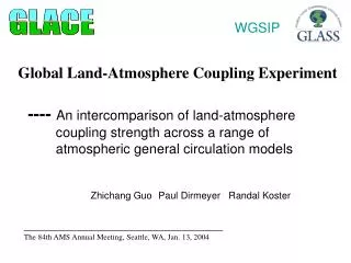
WGSIP. Global Land-Atmosphere Coupling Experiment ---- Model characteristics and comparison Zhichang Guo 1 Paul Dirmeyer 1 Randal Koster 2 1 Center for Ocean-Land-Atmosphere Studies 2 Goddard Space Flight Center, NASA.

E N D
WGSIP Global Land-Atmosphere Coupling Experiment ---- Model characteristics and comparison Zhichang Guo1 Paul Dirmeyer1 Randal Koster2 1 Center for Ocean-Land-Atmosphere Studies 2 Goddard Space Flight Center, NASA __________________________________ The 85th AMS Annual Meeting, San Diego, CA, Jan. 12, 2005
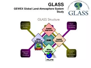
Acknowledgements • GLACE is jointly sponsored by the GEWEX GLASS (Global Land Atmosphere System Study) panel and CLIVAR WGSIP (Working Group on Seasonal-to-Interannual Prediction) • Special thanks are given to the all GLACE participants: Tony Gordon and Sergey Malyshev (GFDL); Yongkang Xue and Ratko Vasic (UCLA); David Lawrence, Peter Cox, and Chris Taylor (HadAM3): Bryant McAvaney (BMRC); Sarah Lu and Ken Mitchell (NCEP/GFS); Diana Verseghy and Edmond Chan (CCCma); Ping Liu (NSIPP); and Eva Kowalczyk and Harvey Davies (CSIRO); Andy Pitman; Taikan Oki and Tomohito Yamada (University of Tokyo ); Yogesh Sud and David M. Mocko (GSFC), Gordon Bonan and Keith W. Oleson (NCAR)
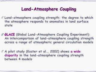
Review • Coupling strength, the extent to which the atmosphere (precipitation, air temperature, etc.) responds to variations in land surface state, is model-dependent. Thus, the results of various land-atmosphere modeling experiments in the literature are also model-dependent. • Koster et al. (2002) show that the strength of the coupling varies significantly among four AGCMs. GLACE (http://glace.gsfc.nasa.gov) is a broad follow-on to this study. 12 international groups participated in GLACE. One paper has been published in Science, and three papers are in preparation for J. Hydrometeorology. • Goal of GLACE: To characterize, using an objective framework, the atmosphere’s response to variations in land variables across a wide range of models. Find out how consistent the models are. Create a “table” of coupling strengths, for better interpretation of the land-atmosphere modeling studies in the literature.
Participating Groups Model Contact Status 1. BMRC with CHASM McAvaney/Pitman submitted 2. U. Tokyo w/ MATSIRO Kanae/Oki submitted 3. COLA with SSiB Dirmeyer/Guo submitted 4. CSIRO w/ 2 land schemes Kowalczyk submitted 5. NCAR Oleson submitted 6. Env. Canada with CLASS Verseghy submitted 7. GFDL with LM2p5 Gordon submitted 8. GSFC(GLA) with SSiB Sud submitted 9. Hadley Centre w/ MOSES2 Taylor/Lawrence submitted 10. NCEP/EMC with NOAH Lu/Mitchell submitted 11. NSIPP with Mosaic Koster submitted 12. UCLA with SSiB Xue submitted
Experiment Design All simulations are run from June through August W Simulations: Establish a time series of surface conditions time step n time step n+1 Step forward the coupled AGCM-LSM Step forward the coupled AGCM-LSM Write the values of the land surface prognostic variables into file W1_STATES Write the values of the land surface prognostic variables into file W1_STATES (Repeat without writing to obtain simulations W2 –16) R Simulations
Experiment Design R Simulations:Run a 16-member ensemble, with each member forced to maintain the same time series of land surface prognostic variables time step n time step n+1 Step forward the coupled AGCM-LSM Step forward the coupled AGCM-LSM Throw out updated values of land surface prognostic variables; replace with values for time step n from files W1_STATES Throw out updated values of land surface prognostic variables; replace with values for time step n+1 from files W1_STATES S Simulations
Experiment Design S Simulations:Run a 16-member ensemble, with each member forced to maintain the same time series of subsurface soil moisture prognostic variables time step n time step n+1 Step forward the coupled AGCM-LSM Step forward the coupled AGCM-LSM Throw out updated values of subsurface soil moisture prognostic variables; replace with values for time step n from file W1_STATES Throw out updated values of subsurface soil moisture prognostic variables; replace with values for time step n+1 from file W1_STATES
Diagnostic Analysis Define a diagnostic variable that describes the impact of the surface boundary on the generation of precipitation. All simulations in ensemble respond to the land surface boundary condition in the same way W (coupling strength) is high intra-ensemble variance is small Simulations in ensemble have no coherent response to the land surface boundary condition W is low intra-ensemble variance is large
Regions with strong coupling strength where 12 participating models are relatively consistent
One major factor: the nature of the evaporation signal, as characterized by the diagnostic sE * (WE(S) – WE(W)) Rationale: The atmosphere is more likely to produce a coherent response to the land surface if the signal it sees at the surface is itself large and coherent. HIGH VALUE OF DIAGNOSTIC: LOW VALUE OF DIAGNOSTIC: E variability high and coherence high E variability low, coherence low E variability high, coherence low E variability low, coherence high
Global Great Plains r2=0.45 r2=0.68 The diagnostic indeed explains much of the intermodel difference in coupling strength. For example, it explains about 70% of the inter-model differences in the Great Plains. The other 30% results from differ-ences in atmospheric parameterization (e.g., convection), sampling error, etc. Northern India Sahel r2=0.63 r2=0.62 coupling strength sE * (WE(S) – WE(W))
Global averages The two factors in the diagnostic, sEandWE(S) – WE(W), can be examined separately. (Evap. variability) (Evap. coherence) WE(S) – WE(W) Coupling strength for BMRC is low due to low evaporation variability Coupling strength for GFS/OSU is low due to low evaporation coherence sE
efficient transmission The evaporation signal is transmitted into precipitation via various parameterizations of atmospheric processes signal transmission strong signal weak signal signal in evaporation inefficient transmission
coupling strength and AGCM parameterizations Evap formulations in these three models might not favor the coupling between sub-surface soil moisture and surface moisture fluxes
coupling strength and AGCM parameterizations Global averages coupling between surface fluxes and precipitation is mostly via convective precipitation scheme in the AGCMs LP CP TP Global averages
Conclusions • Land-atmosphere coupling strength is found to be a function of hydroclimatological regime and is heavily affected by the complex physical process parameterizations implemented in the AGCM. • Impacts of soil moisture on rainfall tend to be strong in the transition zones between dry and wet areas, reflecting the coexistence there of a high ET sensitivity to soil moisture and a high temporal variability of the ET signal.
Conclusions (continued) • The impact of soil moisture on rainfall varies widely from model to model. Most of the intermodel differences in coupling strength can be explained by intermodel differences in the nature of the evaporation signal. • The coupling between surface fluxes and precipitation is mostly via the convective precipitation scheme. Certain ET formulations might not favor the coupling between sub-surface soil moisture and surface moisture fluxes.
Future studies We still need: • An objective quantification of land-atmosphere coupling strength from observational data; • Coupling strength quantified for other seasons; • A more detailed analysis of coupling strength in a more controlled setting, with different configurations of convective precipitation schemes, boundary layer schemes, and ET formulations applied within individual models.