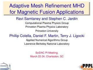
Adaptive Mesh Refinement MHD
Adaptive Mesh Refinement MHD. Ravi Samtaney Computational Plasma Physics Group Princeton Plasma Physics Laboratory Princeton University CEMM Meeting, November 10, Orlando, FL. Collaborators. Phillip Colella, LBNL Steve Jardin, PPPL Terry Ligocki, LBNL Dan Martin, LBNL. Outline.

Adaptive Mesh Refinement MHD
E N D
Presentation Transcript
Adaptive Mesh Refinement MHD Ravi Samtaney Computational Plasma Physics Group Princeton Plasma Physics LaboratoryPrinceton University CEMM Meeting, November 10, Orlando, FL
Collaborators • Phillip Colella, LBNL • Steve Jardin, PPPL • Terry Ligocki, LBNL • Dan Martin, LBNL
Outline • MHD equations and numerical method • Unsplit upwinding method • div(B) issues • Projection method • Semi-implicit MHD code – Progress. • Results • Plane wave propagation • Rotor problem • Magnetic reconnection • Conclusion and future work
Electromagnetic Coupling (courtesy T. Gombosi, Univ. of Michigan) • Weakly coupled formulation • Hydrodynamic quantities in conservative form, electrodynamic terms in source term • Hydrodynamic conservation & jump conditions • One characteristic wave speed (ion-acoustic) • Tightly coupled formulation • Fully conservative form • MHD conservation and jump conditions • Three characteristic wave speeds (slow, Alfvén, fast) • One degenerate eigenvalue/eigenvector
Single-fluid resistive MHD Equations • Equations in conservation form Parabolic Hyperbolic Reynolds no. Lundquist no. Peclet no.
Numerical Method • MHD Equations written in symmetrizable near-conservative form (Godunov, Numerical Methods for Mechanics of Continuum Media, 1, 1972, Powell et al., J. Comput. Phys., vol 154, 1999). • Deviation from total conservative form is of the order of B truncation errors • The symmetrizable MHD equations lead to the 8-wave method. • The fluid velocity advects both the entropy and div(B) • Finite volume approach. Hyperbolic fluxes determined using the unsplit upwinding method (Colella, J. Comput. Phys., Vol 87, 1990) • Predictor-corrector. • Fluxes obtained by solving Riemann problem • Good phase error properties due to corner coupling terms
The r¢ B=0 Problem • Conservation of B =0: • Analytically: if B =0 at t=0 than it remains zero at all times • Numerically: In upwinding schemes the curl and div operators do not commute • Purposes to control B numerically: • To improve accuracy • To improve robustness • To avoid unphysical effects (Parallel Lorentz force) • 8-wave formulation: r¢ B = O(h) (Powell et al, JCP 1999; Brackbill and Barnes, JCP 1980) • Constrained Transport (Balsara & Spicer JCP 1999, Dai & Woodward JCP 1998, Evans & Hawley Astro. J. 1988) • Constrained Transport/Central Difference (Toth JCP 2000) • Projection Method • Vector Potential (Claim: CT/CD schemes can be cast as an “underlying” vector potential. Evans and Hawley, Astro. J. 1988) • Require ad-hoc corrections to total energy • May lead to numerical instability (e.g. negative pressure – ad-hoc fix based on switching between total energy and entropy formulation by Balsara)
r¢B=0 by Projection • Compute the estimates to the fluxes Fn+1/2i+1/2,j using the unsplit formulation • Use face-centered values of B to compute r¢ B. Solve the Poisson equation r2 = r¢ B • Correct B at faces: B=B-r • Correct the fluxes Fn+1/2i+1/2,j with projected values of B • Update conservative variables using the fluxes • The non-conservative source term S(U) r¢ B has been algebraically removed • On uniform Cartesian grids, projection provides the smallest correction to remove the divergence of B. (Toth, JCP 2000) • Does the nature of the equations change? • Hyperbolicity implies finite signal speed • Do corrections to B via r2=r¢ B violate hyperbolicity? • Conservation implies that single isolated monopoles cannot occur. Numerical evidence suggests these occur in pairs which are spatially close. • Corrections to B behave as 1/r2 in 2D and 1/r3 in 3D • Projection does not alter the order of accuracy of the upwinding scheme and is consistent
Adaptive Mesh Refinement with Chombo • Chombo is a collection of C++ libraries for implementing block-structured adaptive mesh refinement (AMR) finite difference calculations (http://www.seesar.lbl.gov/ANAG/chombo) • (Chombo is an AMR developer’s toolkit) • Mixed language model • C++ for higher-level data structures • FORTRAN for regular single grid calculations • C++ abstractions map to high-level mathematical description of AMR algorithm components • Reusable components. Component design based on mathematical abstractions to classes • Based on public-domain standards • MPI, HDF5 • Chombovis: visualization package based on VTK, HDF5 • Layered hierarchical properly nested meshes • Adaptivity in both space and time
Unsplit + Projection AMR Implementation • Implemented the Unsplit method using CHOMBO • Solenoidal B is achieved via projection, solving the elliptic equation r2=r¢ B • Solved using Multgrid on each level (union of rectangular meshes) • Coarser level provides Dirichlet boundary condition for • Requires O(h3) interpolation of coarser mesh on boundary of fine level • a “bottom smoother” (conjugate gradient solver) is invoked when mesh cannot be coarsened • Physical boundary conditions are Neumann d/dn=0 (Reflecting) or Dirichlet • Multigrid convergence is sensitive to block size • Flux corrections at coarse-fine boundaries to maintain conservation • A consequence of this step: r¢ B=0 is violated on coarse meshes in cells adjacent to fine meshes. • Code is parallel • Second order accurate in space and time
Treatment of parabolic flux terms • Approach 1: Explicit • Computed at time step ‘n’ • Magnetic reconnection results use this approach. • Approach 2: Implicit treatment • Implicit Runge Kutta, TGA Approach (Twizell, Gumel, Arigu, Advances in Comp. Math. 6(3):333-352, 1996) • Implemented for resistive terms in magnetic field equations • Work for constant • Viscous and conductivity terms require non-constant coefficient Helmholtz solvers (Work in progress) • Quadratic interpolation (O(h3)) at coarse-fine boundaries • Corner terms required and obtained by linear interpolation • Flux-refluxing step requires implicit solution on all levels synchronized at the current time step. • Backward Euler used for this step
Code verification – Plane wave propagation • A plane wave is initialized oblique to the meshInitial conditions for l-th characteristic waveW(x) = W0(x) + exp(i k¢ x) r_l • Plane wave chosen to correspond to Alfven velocity or fast magnetosonic sound speed • Low (=0.01) • Poisson solve converged in 8 iterations to a max residual of 10-14 • 3D Wave example
Code verification – Weak rotor problem P with B streamlines • Ideal MHD simulation of the “Rotor” problem: high density rotating fluid in a uniform magnetic field. (Balsara and Spicer, J. Comput. Phys. , Vol 149, 1999) • Independent code exists for cross verification (R. Crockett, Astrophysics, UC Berkeley). Detailed comparison in progress.
Code verification – Weak rotor problem with streamlines Conservation Poisson solver convergence history Conservation history
Weak rotor – Resistive MHD (Implicit ) Conservation with velocity streamlines Pressure with B field lines
Magnetic Reconnection: IC and BCs • Initial conditions on domain [-1:1]x[0:1] • Boundary conditionsNo mass flux, (open L/R boundaries)T/B Perfectly conducting wallsDirichlet Temperature BC • Other parameters: Re=103, Pe= 103Dimensionless conductivity and viscosity set to unity • Resitivity variation to annihilate middle island Z-component of B Y-component of B J. Breslau, PhD thesis, Princeton University
Reconnection S= 103 Stage 1Middle islanddecays Stage 2Reconnection Stage 3Decay Bz By Unsplit, B projection, explicit treatment of parabolic fluxes
Reconnection S= 104 6 Level AMR run. Effective unigrid: 4096x2048. Thin O(1/2) high pressure region Super-Alfvenic jets v/a > 4 Reconnection rates show computation is well-resolved
Pressure: Reconnection S= 104 High pressure region shows “patches”. 1.732 1.713 1.669 1.760 1.876 1.942 2.593 1.978 2.253
Current: Reconnection S= 104 Time sequence of current (Jz)Thin current layer “clumps” followedby plasma ejections Asymmetric 1.669 1.713 1.732 1.760 1.876 1.942 2.253 2.593 1.978
. Results:Max scaling with S
Reconnection Energy Budget S=104 S=103
Observations and Conclusion • Observations • Thin current layer well resolved • For S=104 • “patchy” reconnection • Current layer is unstable • Asymmetric evolution after current layer becomes unstable induced by perturbations at mesh level. • Reconnection not a smooth process – bouncing • A conservative solenoidal B AMR MHD code was developed • Unsplit upwinding method for hyperbolic fluxes • r¢ B=0 achieved via projection • This preliminary study indicates that AMR is a viable approach to efficiently resolve the near-singular current sheet in high Lundquist magnetic reconnection
Future Work • High resolution parallel 2D magnetic reconnection runs. • Implicit treatment of viscous/conductivity terms • Two-fluid MHD with Hall effect • Tokamak geometry • Implicit treatment of fast wave • 3D magnetic reconnection • Pellet injection AMR simulations (of importance to ITER and other fusion reactors)
Numerical Method: Finite Volume Approach • Conservative (divergence) form of conservation laws: • Volume integral for computational cell: • Fluxes of mass, momentum, energy and magnetic field entering from one cell to another through cell interfaces are the essence of finite volume schemes. This is a Riemann problem.
Symmetrizable MHD Equations • The symmetrizable MHD equations can be written in a near-conservative form (Godunov, Numerical Methods for Mechanics of Continuum Media, 1, 1972, Powell et al., J. Comput. Phys., vol 154, 1999): • Deviation from total conservative form is of the order of B truncation errors • The symmetrizable MHD equations lead to the 8-wave method. The eigenvalues are • The fluid velocity advects both the entropy and div(B)in the 8-wave formulation
Numerical method: Riemann Solver • The eigenvalues and eigenvectors of the Jacobian, dF/dU are at the heart of the Riemann solver: • Each wave is treated in an upwind manner • The interface flux function is constructed from the individual upwind waves • For each wave the artificial dissipation (necessary for stability) is proportional to the corresponding wave speed • Discontinuous initial condition • Interaction between two states • Transport of mass, momentum, energy and magnetic flux through the interface due to waves propagating in the two media • Riemann solver calculates interface fluxes from left and right states
-U t A3 A1 A4 A2 Unsplit method – Basic concept • Original idea by P. Colella (Colella, J. Comput. Phys., Vol 87, 1990) • Consider a two dimensional scalar advection equation • Tracing back characteristics at t+ t • Expressed as predictor-corrector • Second order in space and time • Accounts for information propagating across corners of zone Corner coupling I II
Unsplit method: Hyperbolic conservation laws • Hyperbolic conservation laws • Expressed in “primitive” variables • Require a second order estimate of fluxes
Unsplit method: Hyperbolic conservation laws • Compute the effect of normal derivative terms and source term on the extrapolation in space and time from cell centers to cell faces • Compute estimates of Fd for computing 1D Flux derivatives Fd / xd - I + I
Unsplit method: Hyperbolic conservation laws • Compute final correction to WI,§,d due to final transverse derivatives • Compute final estimate of fluxes • Update the conserved quantities • Procedure described for D=2. For D=3, we need additional corrections to account for (1,1,1) diagonal couplingD=2 requires 4 Rieman solves per time stepD=3 requires 12 Riemann solves per time step II
The r¢ B=0 Problem • Conservation of B =0: • Analytically: if B =0 at t=0 than it remains zero at all times • Numerically: In upwinding schemes the curl and div operators do not commute • Approaches: • Purist: Maxwell’s equations demand B =0 exactly, so B must be zero numerically • Modeler: There is truncation error in components of B, so what is special in a particular discretized form of B? • Purposes to control B numerically: • To improve accuracy • To improve robustness • To avoid unphysical effects (Parallel Lorentz force)
Approaches to address the r¢B=0 constraint • 8-wave formulation: r¢ B = O(h) (Powell et al, JCP 1999; Brackbill and Barnes, JCP 1980) • Constrained Transport (Balsara & Spicer JCP 1999, Dai & Woodward JCP 1998, Evans & Hawley Astro. J. 1988) • Field Interpolated/Flux Interpolated Constrained Transport • Require a staggered representation of B • Satisfy r¢ B=0 at cell centers using face values of B • Constrained Transport/Central Difference (Toth JCP 2000) • Flux Interpolated/Field Interpolated • Satisfy r¢ B=0 at cell centers using cell centered B • Projection Method • Vector Potential (Claim: CT/CD schemes can be cast as an “underlying” vector potential. Evans and Hawley, Astro. J. 1988) • Require ad-hoc corrections to total energy • May lead to numerical instability (e.g. negative pressure – ad-hoc fix based on switching between total energy and entropy formulation by Balsara)
r¢ B=0 using a Vector Potential • The original 8-wave formulation proved numerically unstable for a 2D reconnection problem (Samtaney et al, Sherwood 2002) • Stability was achieved with a combination of the generalized upwinding (8-wave formulation by Powell et al. JCP vol 154, 284-309, 1999) and vector potential in 2D • Vector potential evolved using central differences • At end of each stage in time integration replace x and y components of B using vector potential • Central difference approximation of div(B) is zero • Issues with vector potential + upwinding approach • Ad-hoc • Loss of accuracy • 3D requires a gauge condition Elliptic problem • Non conservative (but 2D Magnetic reconnection does not exhibit discontinuities)
r¢B=0 by Projection • Compute the estimates to the fluxes Fn+1/2i+1/2,j using the unsplit formulation • Use face-centered values of B to compute r¢ B. Solve the Poisson equation r2 = r¢ B • Correct B at faces: B=B-r • Correct the fluxes Fn+1/2i+1/2,j with projected values of B • Update conservative variables using the fluxes • The non-conservative source term S(U) r¢ B has been algebraically removed • On uniform Cartesian grids, projection provides the smallest correction to remove the divergence of B. (Toth, JCP 2000)
r¢B=0 by Projection • Does the nature of the equations change? • Hyperbolicity implies finite signal speed • Do corrections to B via r2=r¢ B violate hyperbolicity? • Conservation implies that single isolated monopoles cannot occur. Numerical evidence suggests these occur in pairs which are spatially close. • Corrections to B behave as 1/r2 in 2D and 1/r3 in 3D • Projection does not alter the order of accuracy of the upwinding scheme and is consistent
AMR Implementation • CHOMBO framework used for adaptive mesh refinement • Implemented the unsplit method for hyperbolic fluxes • Parabolic fluxes treated explicitly • Quadratic interpolation (O(h3)) at coarse-fine boundaries • Solenoidal B is achieved via projection, solving the elliptic equation r2=r¢ B • Solved using Multgrid on each level (union of rectangular meshes) • Coarser level provides Dirichlet boundary condition for • Requires O(h3) interpolation of coarser mesh on boundary of fine level • a “bottom smoother” (conjugate gradient solver) is invoked when mesh cannot be coarsened • Physical boundary conditions are Neumann d/dn=0 (Reflecting) or Dirichlet • Multigrid convergence is sensitive to block size • Flux corrections at coarse-fine boundaries to maintain conservation • A consequence of this step: r¢ B=0 is violated on coarse meshes in cells adjacent to fine meshes. • Code is parallel • Second order accurate in space and time
Adaptive Mesh Refinement with Chombo • Chombo is a collection of C++ libraries for implementing block-structured adaptive mesh refinement (AMR) finite difference calculations (http://www.seesar.lbl.gov/ANAG/chombo) • (Chombo is an AMR developer’s toolkit) • Mixed language model • C++ for higher-level data structures • FORTRAN for regular single grid calculations • C++ abstractions map to high-level mathematical description of AMR algorithm components • Reusable components. Component design based on mathematical abstractions to classes • Based on public-domain standards • MPI, HDF5 • Chombovis: visualization package based on VTK, HDF5 • Layered hierarchical properly nested meshes • Adaptivity in both space and time
Chombo Layered Design • Chombo layers correspond to different levels of functionality in the AMR algorithm space • Layer 1: basic data layout • Multidimensional arrays and set calculus • data on unions of rectangles mapped onto distributed memory • Layer 2: operators that couple different levels • conservative prolongation and restriction • averaging between AMR levels • interpolation of boundary conditions at coarse-fine interfaces • refluxing to maintain conservation at coarse-fine interfaces • Layer 3: implementation of multilevel control structures • Berger-Oliger time stepping • multigrid iteration • Layer 4: complete PDE solvers • Godunov methods for gas dynamics • Ideal and single-fluid resistive MHD • elliptic AMR solvers