Download
1 / 201
3.12k likes | 4.62k Vues
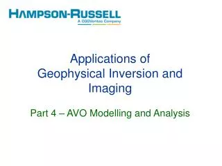
Applications of Geophysical Inversion and Imaging Part 4 – AVO Modelling and Analysis. Introduction. In our previous section on rock physics we discussed fluid effects on P and S-wave velocity, and density. We then looked at post-stack inversion, its advantages and limitations.

E N D
Applications ofGeophysical Inversion and ImagingPart 4 – AVO Modelling and Analysis
Introduction • In our previous section on rock physics we discussed fluid effects on P and S-wave velocity, and density. • We then looked at post-stack inversion, its advantages and limitations. • Next, we considered the recording of S-wave data. • In this section, we will first review the basic principles of AVO and show it’s relationship with P and S-wave velocity. • We will then look at the AVO response of two simple models, one wet and one gas-saturated. • We will then look at various AVO modeling schemes, including full wave equation modeling and anisotropic modeling.
“Bright spots” Recall that in the section on inversion, we showed the “bright spot” shown above, and pointed out that in the 1970’s this would have been interpreted as a gas sand.
The AVO method But “bright spots” can be caused by lithologic variations as well as gas sands. This lead geophysicists in the 1980’s to start looking at pre-stack seismic data. The amplitude increase with offset shown here is an example of a Class 3 sand, as we will discuss later.
Reflected SV-wave = RS(q1) Incident P-wave Reflected P-wave = RP(q1) 1 1 1 VP1 , VS1, r1 VP2 , VS2, r2 2 Transmitted P-wave = TP(q1) 2 Transmitted SV-wave = TS(q1) Mode Conversion Consider the interface between two geologic horizons of differing P and S-wave velocity and density and an incident P-wave at angle q1. This will produce P and S reflected and transmitted waves, as shown above.
Utilizing Mode Conversion But how do we utilize mode conversion? There are actually two ways: • (1) Record the converted S-waves using three-component receivers (in the X, Y and Z directions). This was discussed in the last chapter. • (2) Interpret the amplitudes of the P-waves as a function of offset, or angle, which contain implied information about the S-waves. This is called theAVO (Amplitude versus Offset) method. In the AVO method, we can make use of the Zoeppritzequations, or some approximation to these equations, to extract S-wave type information from P-wave reflections at different offsets.
The Zoeppritz Equations Zoeppritz derived the amplitudes of the reflected and transmitted waves using the conservation of stress and displacement across the layer boundary, which gives four equations with four unknowns. Inverting the matrix form of the Zoeppritz equations gives us the exact amplitudes as a function of angle:
The Aki-Richards Equation The Aki-Richards equation is a linearized approximation to the Zoeppritz equations. The initial form (Richards and Frasier, 1976) separated the velocity and density terms: where:
Wiggins’ version of Aki-Richards A totally equivalent form was derived by Wiggins. He separated the equation into three reflection terms, as follows: where:
Reflectivity approximation To see why the A term in the linearized approximation is approximately equal to the zero-offset reflection coefficient, recall that in Part 2 we showed that: This leads to:
Fatti’s version of Aki-Richards Another equivalent form was derived by Fatti et al. They separated the equation into three reflection terms, as follows:
All three forms of the Aki-Richards equation consist of the sum of three terms, each term consisting of a weight multiplied by an elastic parameter (i.e. a function of VP , VS or r). Here is a summary: A Summary of the Aki-Richards Eq. Equation Weights Elastic Parameters Aki-Richards Wiggins et al. Fatti et al. Note that the weighting terms a, b, c and d, e, f contain the squared VP/VS ratio as well as q. However, in the Wiggins et al. formulation, this term is in the elastic parameter B.
Physical interpretation • A physical interpretation of the three equations is as follows: • Since the seismic trace consists of changes in impedance rather than velocity or density independently, the original form of the Aki-Richards equation is rarely used. • The A, B, C formulation of the Aki-Richards equation is very useful for extracting empirical information about the AVO effect (i.e. A, which is called the intercept, B, called the gradient, and C, called the curvature) which can then be displayed or cross-plotted. Explicit information about the Vp/Vs ratio is not needed in the weights. • The Fatti et al. formulation gives us a way to extract quantitative information about the P and S reflectivity which can then be used for pre-stack inversion. The terms RP0 and RS0 are the linearized zero-angle P and S-wave reflection coefficients.
Wet and Gas Models VP1,VS1, 1 VP2,VS2, 2 Let us now see how to get from the geology to the seismic using the second two forms of the Aki-Richards equation. We will do this by using the two models shown below. Model Aconsists of a wet, or brine, sand, and Model B consists of a gas-saturated sand. VP1,VS1, 1 VP2,VS2, 2 (a) Wet model (b) Gas model
Model Values In the section on rock physics, we computed values for wet and gas sands using the Biot-Gassmann equations. The computed values were: Wet: VP2 = 2500 m/s, VS2= 1250 m/s, 2 = 2.11 g/cc, s2 = 0.33 Gas: VP2= 2000 m/s, VS2= 1310 m/s, 2 = 1.95 g/cc, s2 = 0.12 Values for a typical shale are: Shale: VP1 = 2250 m/s, VS1= 1125 m/s, 1 = 2.0 g/cc, s1 = 0.33 This gives us the following values at the top of the sand/shale zone: Wet Sand: Gas Sand:
Exercise 4-1 Compute the intercept, A, the gradient term, B, and the curvature, C, for the top and base of both the wet model and the gas model, given the parameters on the previous page. Note that the base values are the negative of the top due to symmetry: Wet Model Top: A = B = C = Gas Model Top: A = B = C = Wet Model Base: A = B = C = Gas Model Base: A = B = C =
Exercise 4-2 For both the next exercise and a later exercise on anisotropy effects in AVO, you will need to compute the following trigonometric functions of four angles. Compute them here for later use. sin2q tan2q sin2q*tan2q
Exercise 4-3 Using the A, B, and C terms for the wet and gas models that were computed in Exercise 1, work out the values for R(q) at angles of 0o, 15o, 30o, and 45oin the table below. Then, plot the results on graph paper, with and without the third term, as a function of . Top: Base:
Wet Model AVO Curves 0.2 0.1 RP(q) 0.0 10o 20o 30o 40o 50o - 0.1 - 0.2 q
Gas Model AVO Curves 0.2 0.1 RP(q) 0.0 10o 20o 30o 40o 50o - 0.1 - 0.2 q
Wet Model AVO Curves 0.2 Wet Sand Top 0.1 RP(q) 0.0 10o 20o 30o 40o 50o - 0.1 Wet Sand Base - 0.2 q
Gas Model AVO Curves 0.2 Gas Sand Base 0.1 RP(q) 0.0 10o 20o 30o 40o 50o - 0.1 Gas Sand Top - 0.2 q
Gas Model AVO Curves This figure on the right shows the computed AVO curves for the top and base interfaces of the gas sand using all three terms (A, B, and C) in the Aki-Richards’ equation, and then only the first two terms (A and B). Note the deviation of the two above 25 degrees.
Wet Model AVO Curves This figure on the right shows the computed AVO curves for the top and base interfaces of the wet sand using all three terms (A, B, and C) in the Aki-Richards’ equation, and then only the first two terms (A and B). Note the deviation of the two above 25 degrees.
Her is a comparison of the results from the ABC and Fatti equations for the top of the sands (because of symmetry in this example, the base of sand values are simply these values multiplied by -1): Parameters for ABC and Fatti eqs. Gas Sand: Wet Sand: Note that A and B have the same polarity for the gas sand and opposite polarity for the wet sand, whereas RP0 and RS0 have opposite polarity for the gas sand and the same polarity for the wet sand. The reason for this will be clear later.
Here are computed values for the ABC and Fatti versions of the Aki-Richards equation at angles of 0, 30 and 60 degrees: Aki-Richards values ABC Method Fatti Method Angle/ Sand RP(q) 1st Term 2nd Term 3rd Term 1st Term 2nd Term 3rd Term 0o Gas 0 0 -0.071 0 0 -0.071 -0.071 30o Gas -0.071 -0.060 -0.006 -0.095 -0.042 6x10⁻⁵ -0.137 60o Gas -0.071 -0.181 -0.133 -0.285 -0.125 0.025 -0.385 0o Wet 0.079 0 0 0.079 0 0 0.079 30o Wet 0.079 -0.020 0.005 0.106 -0.040 -0.002 0.064 60o Wet 0.079 -0.060 0.119 0.318 -0.119 -0.061 0.138
Summary of the ABC and Fatti methods • There was a lot of information in the last slide, but the key points are: • The individual terms in each approach are different, but the sum is always identical. • For an angle of zero degrees, the second two terms in both methods are equal to zero, and the scalar on the first term in the Fatti method is equal to one. • In the ABC method, the first term is always the zero offset reflection coefficient, but this is true only at zero angle in the Fatti method. • The third term makes less of a contribution to the sum in the Fatti method than in the ABC method. • The next slides will show the results at all angles.
Zoeppritz vs ABC – Gas Sand ABC method: two term ABC method: three term Zoeppritz This figure on the right shows the AVO curves computed using the Zoeppritz equations and the two and three term ABC equation, for the gas sand model. Notice the strong deviation for the two term versus three term sum. Note: On the next four plots, the curves have been calculated as a function of incident angle and scaled to average angle.
Zoeppritz vs ABC – Wet Sand This figure on the right shows the AVO curves computed using the Zoeppritz equations and the two and three term ABC equation, for the wet sand model. Again, notice the strong deviation for the two term versus three term sum. ABC method: three term Zoeppritz ABC method: two term
Zoeppritz vs Fatti – Gas Sand This figure on the right shows the AVO curves computed using the Zoeppritz equations and the two and three term Fatti equation, for the gas sand model. Notice there is less deviation between the two term and three term sum than with the ABC approach. Zoeppritz Fatti method: two term Fatti method: three term
Zoeppritz vs Fatti – Wet Sand Zoeppritz Fatti method: two term Fatti method: three term This figure on the right shows the AVO curves computed using the Zoeppritz equations and the two and three term Fatti equation, for the wet sand model. As in the gas sand case, there is less deviation between the two term and three term sum than with the ABC approach.
The final synthetic seismogram This final computed synthetic seismogram is shown above on the right, where the log curves are on the left. Notice that the sand is thin enough that the wavelets from the top and bottom of the layer “tune” together.
Ostrander’s Paper • Ostrander (1984) was one of the first to write about AVO effects in gas sands and proposed a simple two-layer model which encased a low impedance, low Poisson’s ratio sand, between two higher impedance, higher Poisson’s ratio shales. • This model is shown in the next slide. • Ostrander’s model worked well in the Sacramento valley gas fields. However, it represents only one type of AVO anomaly (Class 3) and the others will be discussed in the next section.
Ostrander’s Model Ostrander (1984) wrote the classic paper on AVO. His model is shown above. Notice that the model consists of a low acoustic impedance gas sand encased between two shales
Synthetic from Ostrander’s Model (a) Well log responses for the model. (b) Synthetic seismic. Notice that Ostrander’s model produces an increase in amplitude on the pre-stack synthetic gather.
AVO Curves from Ostrander (a) Response from top of model to 45o. (Note that the transmitted P-wave amplitude is shifted to plot within the data range). (b) Response from base of model to 45o.
Ostrander’s case study - stack Ostrander’s case study is from the Sacramento basin. The stack above has “bright spots” at locations A, B, and C, but only A and B are due to gas.
Ostrander’s case study (A) (B) (C) Supergathers from locations A, B, and C. Note that locations A and B show amplitude increases with offset but C does not.
Shuey’s Equation • Shuey (1985) rewrote the Aki-Richards equation using VP, , and , writing the basic form the same way: • Only the gradient is different than in the Aki-Richards expression, and is given by:
Shuey vs Aki-Richards • In this course, we have been using a modeled gas sand and wet sand example. Using Shuey’s equation for this example, we get the following comparison with the answers in exercise 6-1: B (Aki-Richards) B (Shuey) Gas Sand Top: -0.242 -0.252 Wet Sand Top: -0.079 -0.079 • Why do we get the same values in the wet case but not in the gas case?
Shuey vs Aki-Richards This figure shows a comparison between theAki- Richards and Shuey equations for the gas sand we just considered.
Multi-layer AVO modeling Multi-layer modeling in the consists first of creating a stack of N layers, generally using well logs, anddefining the thickness, P-wave velocity, S-wave velocity,and density for each layer. You must then decide what effects are to be includedin the model: primaries only, converted waves, multiples,or some combination of these.
The Possible Modelled Events The following example, taken from Simmons and Backus (AVO Modeling and the locally converted shear wave, Geophysics 59, p1237, August, 1994), illustrates the effect of wave equation modeling. The figure above shows the modelling options.
The Oil Sand Model Simmons and Backus used the thin bed oil sand model shown above.
Response to various algorithms Simmons and Backus (1994) (A) Primaries-only Zoeppritz, (B) + single leg shear, (C) + double-leg shear, (D) + multiples,(E) Wave equation solution, (F) Linearized approximation.
Primary and Converted Waves Zoeppritz, primaries only Aki-Richards, primaries Single leg conversions Zoeppritz, primaries + single leg conversions Simmons and Backus (1994)
Logs from a real data example The logs shown above come from a real data example in the Colony sand that we will look at in the next section.
Models from a Real Data Example (a) Full elastic wave. (b) Zoeppritz equation. (c) Aki-Richards equation.
AVO Modeling Poisson’s ratio Offset Stack P-wave S-wave Density Synthetic Based on AVO theory and the rock physics of the reservoir, we can perform AVO modeling, as shown above. Note that the model result is a fairly good match to the offset stack.
Anisotropy and AVO • So far, we have considered only the isotropic case, in which earth parameters such as velocity do not depend on seismic propagation angle. • In the next few slides, we will discuss anisotropy, in particular the case of Transverse Isotropy with a vertical symmetry axis, or VTI. • We will then see how anisotropy affects the AVO response. • Finally, we will look at this effect on our original model