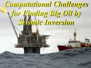
Computational Challenges for Finding Big Oil by Seismic Inversion
490 likes | 704 Vues
Computational Challenges for Finding Big Oil by Seismic Inversion. Motivation for Better Seismic Imaging Strategy. Jack Buckskin. ¼ billion $$$ well. 35,055 Feet. Kaskida Tiber. Motivation for Better Seismic Imaging Strategy Oil Well Blowouts.

Computational Challenges for Finding Big Oil by Seismic Inversion
E N D
Presentation Transcript
Computational Challenges for Finding Big Oil by Seismic Inversion
Motivation for Better Seismic Imaging Strategy Jack Buckskin ¼ billion $$$ well 35,055Feet Kaskida Tiber
Motivation for Better Seismic Imaging Strategy Oil Well Blowouts
Motivation for Better Seismic Imaging Strategy Oil Well Blowouts Overpressure Zone = Low Seismic Velocity Zone
Motivation for Better Seismic Imaging Strategy Mud Volcanoes May 29, 2006 13 people killed 30,000 people displaced 2 6.3 km
Outline • Computational Challenge Seismic Inversion • Full waveform Inversion • Multisource Inversion
Seismic Inverse Problem 2 Soln: min || Lm-d || migration waveform inversion -1 T T m = [L L] L d T L d Given: d= Lm Find: m(x,y,z)
Computational Challenges -1 T T m = [L L] L d Given: d= Lm Find: d > 10 13 words 7 m > 10 3 20x20x10 km unknown velocity values 4 dx=1 m # time steps ~ 10 4 # shots > 10 Total = 15 10
Outline • Computational Challenge Seismic Inversion • Full waveform Inversion • Multisource Inversion
Nd +Nd =[NL +NL ]m 1 1 2 2 1 1 2 2 mmig=LTd Multisource Migration: m =[LTL]-1LTd Multisrc-Least FWI: multisource preconditioner Preconditioned m’ = m - LT[Lm - d] f Steepest Descent f ~ [LTL]-1 Multisource Encoded FWI Forward Model:
syn. 2. Generate synthetic data d(x,t) by FD method syn. 2 3. Adjust v(x,z) until ||d(x,t)-d(x,t) || minimized by CG. mute b). Use multiscale: low freq. high freq. Multiscale Waveform Tomography 1. Collect data d(x,t) 4. To prevent getting stuck in local minima: a). Invert early arrivals initially 7
Boonyasiriwat et al., 2009, TLE 0 km 6 km/s 6 km 3 km/s 0 km 20 km
Waveform Tomograms 0 km 6 km/s Initial model 6 km 3 km/s 0 km 5 Hz 6 km/s 6 km 3 km/s 0 km 6 km/s 10 Hz 6 km 3 km/s 0 km 6 km/s 20 Hz 6 km 3 km/s 0 km 20 km
Low-pass Filtering (b) 0-15 Hz CSG (c) 0-25 Hz CSG 18
Dynamic Early-Arrival Muting Window Window = 1 s Window = 1 s 0-15 Hz CSG 0-25 Hz CSG 19
Dynamic Early-Arrival Muting Window Window = 2 s Window = 2 s 0-15 Hz CSG 0-25 Hz CSG 19
Traveltime Tomogram Results 0 Depth (km) 3000 2.5 Velocity (m/s) Waveform Tomogram 0 1500 Depth (km) 2.5 0 X (km) 20 20
3000 Waveform Tomogram 0 Velocity (m/s) Depth (km) 1500 2.5 Vertical Derivative of Waveform Tomogram 0 Depth (km) 2.5 21 0 X (km) 20
Outline • Computational Challenge Seismic Inversion • Full waveform Inversion • Multisource Inversion
Multisource Seismic Imaging vs CPU Speed vs Year 100000 10000 copper 1000 Aluminum VLIW Speed 100 Superscalar 10 RISC 1 1970 1980 1980 1990 2000 2010 2020 Year
FWI Problem & Possible Soln. Problem: FWI computationally costly Solution: Multisource Encoded FWI Preconditioning speeds up by factor 2-3 Iterative encoding reduces crosstalk
Ld +L d 1 2 2 1 = L d +L d + =[L +L ](d + d ) 1 2 1 2 1 1 2 2 d +d =[L +L ]m 1 2 1 2 mmig=LTd Multisource Migration: Multisource Phase Encoded Imaging { { L d Forward Model: T T T T T T m = m + (k+1) (k) Crosstalk noise Standard migration
Multi-Source Waveform Inversion Strategy (Ge Zhan) 144 shot gathers Generate multisource field data with known time shift Initial velocity model Generate synthetic multisource data with known time shift from estimated velocity model Multisource deblurring filter Using multiscale, multisource CG to update the velocity model with regularization
3D SEG Overthrust Model(1089 CSGs) 15 km 3.5 km 15 km
Numerical Results Dynamic QMC Tomogram (99 CSGs/supergather) Static QMC Tomogram (99 CSGs/supergather) 3.5 km Dynamic Polarity Tomogram (1089 CSGs/supergather) 15 km
Multisource FWI Summary (We need faster migration algorithms & better velocity models) Stnd. FWI Multsrc. FWI IO 1 vs 1/20 Cost 1 vs 1/20 or better Sig/MultsSig ? Resolution dx 1 vs 1
Multisource FWI Summary (We need faster migration algorithms & better velocity models) Future: Multisource MVA, Interpolation, Field Data, Migration Filtering, LSM
Research Goals G.T. Schuster (Columbia Univ.,1984) Shaheen Seismic Interferometry: VSP, SSP, OBS Multisource+PreconditionedRTM+MVA+Inversion+Modeling: TTI 3D RTM, GPU: Stoffa+CSIM, UUtah K. Johnson SCI, PSU, KAUST Cornea
Multisource S/N Ratio L [d + d +.. ] d , d , …. d +d +…. L [d + d + … ] T T 2 1 2 1 2 2 1 1 # CSGs # geophones/CSG
Multisrc. Migration vs Standard Migration # geophones/CSG # CSGs MS MS MI vs MS M ~ ~ S-1 Iterative Multisrc. Migration vs Standard Migration # iterations vs
Ld +L d 1 2 2 1 Crosstalk Term T T Time Statics Time+Amplitude Statics QM Statics
Ld +L d 1 2 2 1 Summary T T Time Statics 1. Multisource crosstalk term analyzed analytically 2. Crosstalk decreases with increasing w, randomness, dimension, iteration #, and decreasing depth Time+Amplitude Statics 3. Crosstalk decrease can now be tuned QM Statics 4. Some detailed analysis and testing needed to refine predictions.
Multisource Technology • Fast Multisource Least Squares Kirchhoff Mig. • Multisource Waveform Inversion (Ge Zhan)
The Marmousi2 Model 0 Z k(m) 3 0 X (km) 16 The area in the white box is used for S/N calculation.
Conventional Source: KM vs LSM (50 iterations) 0 Z k(m) KM (1x) 3 0 X (km) 16 0 Z (km) LSM (100x) 3 0 X (km) 16
200-source Supergather: KM vs LSM (300 its.) 0 Z k(m) KM (1/200x) 3 0 X (km) 16 0 Z (km) LSM (33x) 3 0 X (km) 16
S/N = The S/N of MLSM image grows as the square root of the number of iterations. MI 7 S/N 0 300 1 I
Multisource Technology • Fast Multisource Least Squares Migration ( Dai) • Multisource Waveform Inversion (Boonyasiriwat)
Comparing CIGs CIG from Waveform Tomogram CIG from Traveltime Tomogram 24
Comparing CIGs CIG from Waveform Tomogram CIG from Traveltime Tomogram 26
Comparing CIGs CIG from Waveform Tomogram CIG from Traveltime Tomogram 28
Data Pre-Processing 3D-to-2D conversion Attenuation compensation Random noise removal 17
Source Wavelet Estimation Generate a stacked section Pick the water-bottom Stack along the water-bottom to obtain an estimate of source wavelet In some cases, source wavelet inversion can be used. 17
Gradient Computation and Inversion Multiscale inversion: low to high frequency Dynamic early-arrival muting window Normalize both observed and calculated data within the same shot Quadratic line search method (Nocedal and Wright, 2006) A cubic line search can also be used. 17