Overview of Multisource Phase Encoded Seismic Inversion
540 likes | 746 Vues
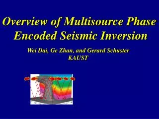
Overview of Multisource Phase Encoded Seismic Inversion. Wei Dai, Ge Zhan, and Gerard Schuster KAUST. Outline. Seismic Experiment:. L m = d. 1. 1. L m = d. 2. 2. L m = d. . . N. N. . 2. Standard vs Phase Encoded Least Squares Soln. L. d. 3. Theory Noise Reduction.

Overview of Multisource Phase Encoded Seismic Inversion
E N D
Presentation Transcript
Overview of Multisource Phase Encoded Seismic Inversion Wei Dai, Ge Zhan, and Gerard Schuster KAUST
Outline Seismic Experiment: Lm = d 1 1 Lm = d 2 2 Lm = d . . N N . 2. Standard vs Phase Encoded Least Squares Soln. L d 3. Theory Noise Reduction ]m = [N d + N d ] vs [ N L + N L 1 1 m = L d 2 2 2 2 1 1 1 1 2 2 4. Summmary and Road Ahead
Gulf of Mexico Seismic Survey Lm = d Predicted data Observed data 4 Common Shot Gather Goal: Solve overdetermined System of equations for m Time (s) 0 d Streamer Reel 4 km Streamer Cables m(x,y,z)
Details of Lm = d 4 d 1 Time (s) 0 6 X (km) Reflectivity or velocity model G(s|x)G(x|g)m(x)dx = d(g|s) Predicted data = Born approximation Solve wave eqn. to get G’s m
Outline Seismic Experiment: Lm = d 1 1 Lm = d 2 2 Lm = d . . N N . 2. Standard vs Phase Encoded Least Squares Soln. L d 3. Theory Noise Reduction ]m = [N d + N d ] vs [ N L + N L 1 1 m = L d 2 2 2 2 1 1 1 1 2 2 4. Summmary and Road Ahead
Conventional Least Squares Solution: L= & d = L d 1 1 L d Given: Lm=d 2 2 In general, huge dimension matrix Find: m s.t. min||Lm-d|| 2 Solution: m = [L L] L d -1 T T or if L is too big m = m – aL (Lm - d) (k+1) (k) (k) T (k) = m – aL (L m - d ) (k) [ ] T + L (L m - d ) T 1 1 1 2 2 2 Problem: L is too big for IO bound hardware
Conventional Least Squares Solution: L= & d = L d 1 1 L d Given: Lm=d 2 2 In general, huge dimension matrix Find: m s.t. min||Lm-d|| 2 Solution: m = [L L] L d -1 T T or if L is too big m = m – aL (Lm - d) (k+1) (k) (k) T (k) = m – aL (L m - d ) (k) [ ] T + L (L m - d ) T 1 1 1 2 2 2 Note: subscripts agree Problem: L is too big for IO bound hardware
Conventional Least Squares Solution: L= & d = L d 1 1 L d Given: Lm=d 2 2 In general, huge dimension matrix Find: m s.t. min||Lm-d|| 2 Solution: m = [L L] L d -1 T T m = m – aL (Lm - d) (k+1) (k) (k) T (k) = m – aL (L m - d ) (k) [ ] T + L (L m - d ) T 1 1 1 2 2 2 Problem: Each prediction is a FD solve Solution: Blend+encode Data Problem: L is too big for IO bound hardware
Blending+Phase Encoding Blending Blending Phase Phase d d d Lm= Lm= Lm= 1 1 3 2 2 3 O(1/S) cost! Encoding Matrix Supergather d = N d + N d + N d 1 1 2 3 2 3 L = Encoded supergather modeler NL + N L + NL m [ ]m 1 2 3 1 2 3
Blended Phase-Encoded Least Squares Solution L =&d = N d + N d N L + N L 1 2 1 1 1 2 2 2 Given: Lm=d In general, SMALL dimension matrix Find: m s.t. min||Lm-d|| 2 Solution: m = [LL] Ld -1 T T or if L is too big m = m – aL (Lm - d) T (k+1) (k) (k) (k) = m – aL (L m - d ) (k) [ ] T + L (L m - d ) T 1 1 1 2 2 2 Iterations are proxy For ensemble averaging + Crosstalk + L (L m - d ) + L (L m - d ) T T 2 1 1 2 1 2
Brief History Multisource Phase Encoded Imaging Migration Romero, Ghiglia, Ober, & Morton, Geophysics, (2000) Waveform Inversion and Least Squares Migration Krebs, Anderson, Hinkley, Neelamani, Lee, Baumstein, Lacasse, SEG, (2009) Virieux and Operto, EAGE, (2009) Dai, and Schuster, SEG, (2009) Biondi, SEG, (2009)
Outline Seismic Experiment: Lm = d 1 1 Lm = d 2 2 Lm = d . . N N . 2. Standard vs Phase Encoded Least Squares Soln. L d 3. Theory + Numerical Results ]m = [N d + N d ] vs [ N L + N L 1 1 m = L d 2 2 2 2 1 1 1 1 2 2 4. Summmary and Road Ahead
Z (km) 0 SEG/EAGE Salt Reflectivity Model 1.4 Use constant velocity model with c = 2.67 km/s Center frequency of source wavelet f = 20 Hz 320 shot gathers, Born approximation 0 6 X (km) • Encoding: Dynamic time, polarity statics + wavelet shaping • Center frequency of source wavelet f = 20 Hz • 320 shot gathers, Born approximation
Standard Phase Shift Migration vs MLSM (Yunsong Huang) Standard Phase Shift Migration (320 CSGs) 0 1 x Z k(m) 1.4 0 X (km) 6 Multisource PLSM (320 blended CSGs, 7 iterations) 0 Z (km) 1 x 44 1.4 0 X (km) 6
Single-source PSLSM (Yunsong Huang) 1.0 Conventional encoding: Polarity+Time Shifts Model Error Unconventional encoding 0.3 0 Iteration Number 50
Multi-Source Waveform Inversion Strategy (Ge Zhan) 144 shot gathers Generate multisource field data with known time shift Initial velocity model Generate synthetic multisource data with known time shift from estimated velocity model Multisource deblurring filter Using multiscale, multisource CG to update the velocity model with regularization
3D SEG Overthrust Model(1089 CSGs) 15 km 3.5 km 15 km
Numerical Results 300x Dynamic QMC Tomogram (99 CSGs/supergather) 300x Static QMC Tomogram (99 CSGs/supergather) 3.5 km Dynamic Polarity Tomogram (1089 CSGs/supergather) 15 km 1000x
Outline Seismic Experiment: Lm = d 1 1 Lm = d 2 2 Lm = d . . N N . 2. Standard vs Phase Encoded Least Squares Soln. L d 3. Theory + Numerical Results ]m = [N d + N d ] vs [ N L + N L 1 1 m = L d 2 2 2 2 1 1 1 1 2 2 4. Summmary and Road Ahead
d +d =[L +L ]m 1 2 1 2 mmig=LTd Multisource Migration: Multisource Least Squares Migration { { L d Forward Model: Phase encoding Kirchhoff kernel Standard migration Crosstalk term 34
Multisource Least Squares Migration Crosstalk term
Crosstalk Prediction Formula ~ X = O( ) 2 2 e -s w X .01 1.0 s L (L m - d ) + L (L m - d ) T T 2 1 1 2 1 2
~ ~ 1 GI G GS [S(t) +N(t) ] S S Standard Migration SNR Zero-mean white noise Assume: d(t) = Standard Migration SNR Neglect geometric spreading GS Cost ~ O(S) # CSGs # geophones/CSG + + + Iterative Multisrc. Mig. SNR Cost ~ O(I) Standard Migration SNR SNR= # iterations migrate stack migrate iterate . SNR= . . SNR=
The SNR of MLSM image grows as the square root of the number of iterations. 7 GI SNR = SNR 0 300 1 Number of Iterations
Summary L d 1 1 m = ]m = [N d + N d ] N L + N L [ L d 2 2 2 2 1 1 1 1 2 2 Stnd. MigMultsrc. LSM IO 1 1/320 1 <1/44 Cost ~ Less 1 1 SNR~ Resolution dx 1 1 Cost vs Quality
Multisource FWI Summary (We need faster migration algorithms & better velocity models) Future: Multisource MVA, Interpolation, Field Data, Migration Filtering, LSM Issues: Optimal encoding strategies, data compression, loss of information.
Summary (We need faster migration algorithms & better velocity models) Stnd. FWI Multsrc. FWI IO 1 vs 1/20 or better Cost 1 vs 1/20 or better Sig/MultsSig ? Resolution dx 1 vs 1
d +d =[L +L ]m 1 2 1 2 mmig=LTd Multisource Migration: Multisource Least Squares Migration { { L d Forward Model: Phase encoding Kirchhoff kernel Standard migration Crosstalk term 34
Multisource Least Squares Migration Crosstalk term
Numerical Result of Multi-source Super stacking (Xin Wang) Narrowed Spectrum Wavelet Reflectivity model 0.4 0 Amplitude Z (km) -0.3 1.4 0 time (s) 0.5 0 X (km) 5.9 KM of 320 Single Source CSG FT of Wavelet 4.5 0 Z (km) Dominant frequency Signal 1.4 0 0 50 Frequency (Hz) X (km) 0 5.9 0.5
Numerical Result of Multi-source Super stacking (Xin Wang) KM of 320 Shots Supergather with PE KM of 320 Shots Supergather w/o PE 0 0 Z (km) Signal + Noise Z (km) Singal + Noise 1.4 1.4 0 X (km) 5.9 0 X (km) 5.9 KM of 3000 Stacking Supergather Gaussian Distribution 4000 50 0 320 320 × 3000 Z (km) Singal + Noise 1.4 0 0 0 0.05 -0.05 -0.05 X (km) 0.05 5.9
Numerical Result of Multi-source Super stacking (Xin Wang) = Signal + Noise Noise − Signal = < N (g,s) N (g,s’)* > if s≠s’ Crosstalk damping coefficient R (σ) / R (σ0) 2 2 2 = e 2ω (σ0- σ ) = Σ Σ Γ(g,x,s)* D0 (g|s) + R Σ Σ Σ Γ (g,x,s)* D0 (g|s’) g s g s≠s’ s 2 R = e-2ω σ 2
The Marmousi2 Model (Wei Dai) 0 Z k(m) 3 0 X (km) 16 The area in the white box is used for SNR calculation. 200 CSGs. Born Approximation Conventional Encoding: Static Time Shift & Polarity Statics
Conventional Source: KM vs LSM (50 iterations) Conventional KM 0 Z k(m) 1x 3 0 X (km) 16 Conventional KLSM 0 50x Z (km) 3 0 X (km) 16
200-source Supergather: Multisrc. KM vs LSM Multisource KM (1 iteration) 0 1 x Z k(m) 200 3 0 X (km) 16 Multisource KLSM (300 iterations) 0 Z (km) 3 0 X (km) 16
Outline 1. Migration Problem and Encoded Migration 2. Standard vs Monte Carlo Least Squares Soln. L d ]m = [N d + N d ] vs [ N L + N L 1 1 m = L d 2 2 2 2 1 1 1 1 3. Numerical Results: Kirchhoff, Phase Shift, RTM 2 2 4. Summary
Z (km) 0 SEG/EAGE Salt Reflectivity Model 1.4 Use constant velocity model with c = 2.67 km/s Center frequency of source wavelet f = 20 Hz 320 shot gathers, Born approximation 0 6 X (km) • Encoding: Dynamic time, polarity statics + wavelet shaping • Center frequency of source wavelet f = 20 Hz • 320 shot gathers, Born approximation
Standard Phase Shift Migration vs MLSM (Yunsong Huang) Standard Phase Shift Migration (320 CSGs) 0 1 x Z k(m) 1.4 0 X (km) 6 Multisource PLSM (320 blended CSGs, 7 iterations) 0 Z (km) 1 x 44 1.4 0 X (km) 6
Single-source PSLSM (Yunsong Huang) 1.0 Conventional encoding: Polarity+Time Shifts Model Error Unconventional encoding 0.3 0 Iteration Number 50
Outline 1. Migration Problem and Encoded Migration 2. Standard vs Monte Carlo Least Squares Soln. L d ]m = [N d + N d ] vs [ N L + N L 1 1 m = L d 2 2 2 2 1 1 1 1 3. Numerical Results: Kirchhoff, Phase Shift, RTM 2 2 4. Summary
3D SEG Overthrust Model(1089 CSGs, Chaiwoot) 15 km 3.5 km 15 km
Numerical Results (Chaiwoot Boonyasiriwat) 300x Dynamic QMC Tomogram (99 CSGs/supergather) 300x Static QMC Tomogram (99 CSGs/supergather) 3.5 km Dynamic Polarity Tomogram (1089 CSGs/supergather) 15 km 1000x
What have we empirically learned? Stnd. MigMultsrc. LSM IO 1 1/320 1 1/44 Cost ~ I=7 S=320 SNR~ Resolution dx 1 1/2 Cost vs Quality: Can I<<S? Yes.
Outline 1. Migration Problem and Encoded Migration 2. Standard vs Monte Carlo Least Squares Soln. L d ]m = [N d + N d ] vs [ N L + N L 1 1 m = L d 2 2 2 2 1 1 1 1 3. Numerical Results 2 2 4. S/N Ratio
~ ~ 1 GI G GS [S(t) +N(t) ] S S Standard Migration SNR Zero-mean white noise Assume: d(t) = Standard Migration SNR Neglect geometric spreading GS Cost ~ O(S) # CSGs # geophones/CSG + + + Iterative Multisrc. Mig. SNR Cost ~ O(I) Standard Migration SNR SNR= # iterations migrate stack migrate iterate . SNR= . . SNR=
The SNR of MLSM image grows as the square root of the number of iterations. 7 GI SNR = SNR 0 300 1 Number of Iterations
Summary L d ]m = [N d + N d ] vs [ N L + N L 1 1 m = L d 2 2 2 2 1 1 1 1 2 2 GS GI Stnd. MigMultsrc. LSM IO 1 1/100 S I Cost ~ SNR Resolution dx 1 1/2 Cost vs Quality: Can I<<S?
Outline Motivation Multisource LSM theory Signal-to-Noise Ratio (SNR) Numerical results Conclusions
ConclusionsMigvs MLSM 1. SNR: VS GS GI 2. Memory 1 vs1/S 2. Cost: S vsI 3. Caveat: Mig. & Modeling were adjoints of one another. LSM sensitive starting model 4. Unconventional encoding: I << S • Next Step: Sensitivity analysis to starting model
Back to the Future? Evolution of Migration 1960s-1970s 1980s 1980s-2010 2010? Poststack migration Prestack migration Poststack encoded migration DMO