Download
1 / 70
720 likes | 806 Vues
Delve into the fundamental equations governing climate models, exploring momentum conservation, forces in the atmosphere, Coriolis effect, and more. Gain insights into current climate phenomena like El Niño and global warming.

E N D
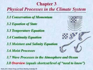
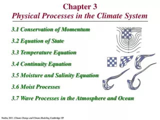
Chapter 3Physical Processes in the Climate System 3.1 Conservation of Momentum 3.2 Equation of State 3.3 Temperature Equation 3.4 Continuity Equation 3.5 Moisture and Salinity Equation 3.6 Moist Processes 3.7 Wave Processes in the Atmosphere and Ocean Neelin, 2011. Climate Change and Climate Modeling, Cambridge UP
Let’s start the discussion with the conservation of momentum MOTIVATION: Climate models are based on these equations and relationships We can use the main balances to understand features of current climate, El Niño, global warming,.. What do I need to know: What we do with the balances & concepts Neelin, 2011. Climate Change and Climate Modeling, Cambridge UP
Figure 3.1 Schematic of directions and velocities Coordinate system for directions and velocities. Blown up region shows local Cartesian coordinate system (for each region of the sphere). Distances east, north & up are x, y, z. (Also lat, lon j, l) Velocity components u, v, w(eastward, northward, up). Neelin, 2011. Climate Change and Climate Modeling, Cambridge UP
Forces in the Atmosphere • Equation of motion: (First and second Laws of Newton) • Real forces (independent on the rotating system): gravity, pressure gradient force and frictional force • Apparent forces due to rotation: apparent centrifugal force (affects gravity) and Coriolis (correction for horizontal movements).
Apparent forces: • Centrifugal force: • Where RA is vector perpendicular to axis of rotation and is angular velocity of earth • Combine with gravity to define "effective" gravity • What this equation means is that the apparent gravity depends on where the body is on earth Note that RA is maximum at the equator: the largest possible centrifugal force: minimum effective gravity: explains why rockets are launched at low latitudes
Coriolis force animation Neelin, 2011. Climate Change and Climate Modeling, Cambridge UP
Coriolis force: Ω At rest over the Earth surface will have cetrifugal acceleration= Ω2R. Suppose it moves eastward with speed u: the centrifugal force would increase to: Centrifugal force= R
Coriolis force: Expanding the equation we have now: Coriolis Force Synoptic scale motions u<< ΩR: Last term can be neglected in a first approximation Centrifugal force due to rotation of the Earth (independent of the relative velocity Deflecting forces that act outward along the vector R
Coriolis force can be divided into vertical and meridional components : R φ To the right of the movement in the NH φ A relative motion along the east-west coordinate will produce an acceleration in the north-south direction given by: And vertical acceleration given by:
Why earth’s angular momentum is higher in low latitudes? Two hours later… Solid earth rotates from W-E with angular speed Ω U=ΩR Both individuals are at the same longitude and same latitudes as before However, angular momentum is larger at the equator – linear momentum larger Both individuals are at the same longitude, different latitudes
Suppose now that a particle initially at rest on the Earth is set in motion equatoward by impulsive forces As it moves equatorward it will conserve its angular momentum in the absence of torques: a relative westward velocity must develop Ω R a R + δR If we expand the right hand side and neglect second order differentials (and assume that δR<<R and solve for δu, we get: a= Earth’s Radius
In summary If we define the Coriolis parameter f as: The relative horizontal motion produces a horizontal acceleration perpendicular to the movement given by: NH:v <0, f>0 then the parcels will experience a negative increment in u (Eq.1) (easterly component) TRADE WINDS SH: v >0, f<0 then the parcels will experience a negative increment in u (Eq. 1) (easterly component) U zonal <0
Likewise… NH: u > 0, f>0 then the parcels will experience a negative increment in v (Eq.1) (northerly component) SH: u > 0, f<0 then the parcels will experience a positive increment in v (Eq.1) (southerly component)
df dy Coriolis force (cont.) f is very small (varies from ~10-4 (high lat) to 10-5 seg-1 in tropics Therefore: it is negligible for movements with time scales short compared to the rotation of the earth (cloud movements, sea breeze (if not lasting too long) “Beta effect” change of Coriolis force with latitude • is proportional to cos(latitude) • Always positive and maximum at the equator • matters because Coriolis so important Neelin, 2011. Climate Change and Climate Modeling, Cambridge UP
REMEMBER THAT A “GRADIENT” ALWAYS POINTS TOWARD THE HIGHEST MAGNITUDES OF THE SCALAR. wind direction Pressure Gradient Force z Pressure Gradient y High Pressure p1 Low Pressure p2 >0 for sure x Hydrostatic Equation: Definition of Geopotential Geopotential Height See Holton, 1979, second Ed. Chap1, pg. 21
Surface of constant Pressure Changes in geopotential height Changes in geopotential height imply in the existence of pressure gradient forces
Winds and geopotential height: example: sea breeze High Pressure LAND OCEAN W E
Friction or Viscosity Force τis the shear stress and is the rate of vertical exchange of horizontal momentum N/m2 τs at the surface
d dt velocity = Coriolis+PGF+gravity+FdragEq. 3.2 dv du 1 1 ¶p ¶p _ + Fdrag + Fdrag y x = fv ¶x ¶y dt dt _ _ = fu Horizontal momentum equations (Horizontal = perpendicular to gravity) x-direction (east) Eq. 3.4 y-direction (north) Eq. 3.5 Largest terms (usually) Neelin, 2011. Climate Change and Climate Modeling, Cambridge UP
In a tangent plan we have (this is important to remember): We can eliminate density by using the relationship between pressure gradient and geopotential Remember that Friction is defined as a negative component that is supposed to decrease (decelerate) the speed
Geostrophic winds L 5460m FGP FGP FGP wind FGP FGP 5560m CF CF CF 5640m CF H Estimate the geostrophic winds given this distribution of geopotential height, assuming that the spatial interval between the two lines is equal 100km. Assume this region is in midlatitudes of the NH
500mb chart Geostrophic balance is observed where the isolines of geop. are parallel
Gradient Wind • Curved trajectories when the wind direction is changed: the centripetal (or centrifugal) acceleration needs to be considered in the balance of forces • Centripetal acceleration is given by: V2/RT, where RT is the local radius of curvature of the air trajectories. The signs of these terms depend on the curvature
Since Co is dependent on the wind speed, and since the centrifugal force is in the same direction as Co, the balance of forces can be achieved at slower speeds compared with a geostrophic one : SUBGEOSTROPHIC The centrifugal force is opposite to Co: Balance is achieved at higher speeds compared with the geostrophic balance: SUPERGEOSTROPHIC WINDS The centrifugal force Acts in the same direction as Coriolis
Tridimensional view Northern Hemisphere
Vertical movement in p-coordinates • The vertical velocity component in (x,y,p) coordinate is V- horizontal wind • Substituting (δp/ δz )=-ρg from the Hydrostatic equation: Note that w and ω have opposite sign: ascending (descending) movements ω negative (positive) ~ 1 week for a parcel to move from the lower to the upper troposphere 10hPa/day <<10hPa/day 100hPa/day
How to interpret ω Pressure ω=dp/dt 600mb 700mb 800mb 900mb 1000mb
Comparing w with ω • 100hPa/day is equivalent to 1km/day or 1cm/s in the lower troposphere and twice that value in the midtroposphere (the distance between two pressure levels increases with height)
3.4 Continuity equation Diverging motions Figure 3.7 3-D divergence e.g., ocean sfc. • Conservation of mass: mass = density • volume • Divergence in 3 dimensions D3D rate of change of volume would tend to reduce density • Ocean case: hard to change density much • Horizontal divergence balanced by vertical motions } Neelin, 2011. Climate Change and Climate Modeling, Cambridge UP
= -D3D ∂v ∂u d ∂y ∂x dt D = + 3.4 Continuity equation ] [Details: full eqn. Eq. 3.28 3.4.1 Oceanic continuity equation Horizontal divergence: Eq. 3.30 ∂w Eq. 3.29 D = - Ocean approx. ∂z • Horizontal divergence balanced by net inflow in vertical Neelin, 2011. Climate Change and Climate Modeling, Cambridge UP
∂ ∂p _ D = 3.4.2 Atmospheric continuity equation • Atmospheric continuity eqn.: simple in pressure coord. • recall pressure surfaces are mass surfaces • Horizontal divergence D along pressure surfaces must be balanced by vertical motion [ Eq. 3.31 • vertical velocity in pressure coord.] • e.g., low level convergence balanced by rising motion • [Note pressure increases downward so is negative for rising motions] Neelin, 2011. Climate Change and Climate Modeling, Cambridge UP
drag fu ≈ Fy _ ∂w D = ∂z Coastal upwelling: e.g., Peru; northward wind component along a north-south coast • Drag of wind stress tends to accelerate currents northward • Coriolis force turns current to left in S. Hem • [momentum eqn. ] • u away from coast horizontal divergence upwelling from below[thru bottom of surface layer ≈ 50m] • [Continuity eqn. ] Figure 3.9 Neelin, 2011. Climate Change and Climate Modeling, Cambridge UP
Figure 3.10 Processes leading to equatorial upwelling • Wind stress accelerates currents westward • [wind speed fast relative to currents, so frictional drag at surface slows the wind but accelerates the currents] • Just north of Equator small Coriolis force turns current slightly to right (south of Equator to the left) Þ divergence in surface layer Þ balanced by upwelling from below Neelin, 2011. Climate Change and Climate Modeling, Cambridge UP
Section 3.1 Overview An approximate balance between the Coriolis force and the pressure gradient force holds for winds and currents in many applications (geostrophic balance) (Fig. 3.4). The Coriolis force tends to turn a flow to the right of its motion in the Northern Hemisphere (left in the Southern Hemisphere); the pressure gradient force acts from high toward low pressure. The Coriolis parameterf varies with latitude (zero at the equator, increasing to the north, negative to the south); this is called the beta-effect ( = rate of change of f with latitude). In the vertical direction, the pressure gradient forcebalancesgravity (hydrostatic balance). This allows us to use pressure as a vertical coordinate. Pressure is proportional to the mass above in the atmospheric or oceanic column. Neelin, 2011. Climate Change and Climate Modeling, Cambridge UP
Figure 3.5 Application: thermal circulation • UCSB (sea breeze) SM Bay Tropics (Hadley circ) subtropics • West Pacific (Walker circ.) East Pacific • relatively low pressure (at given height) at low levels in warm region; PGF toward warm region (near surface) e.g.: Neelin, 2011. Climate Change and Climate Modeling, Cambridge UP
hydrostatic + ideal gas law gives: • fixed mass per area between pressure surfaces • Warm air less dense greater column thickness (height difference) between two pressure surfaces • p1 below z1 in warm region, so p at z1 is L rel to cool region Neelin, 2011. Climate Change and Climate Modeling, Cambridge UP
3.7 Wave Processes in the Atmosphere and Ocean: Overview • Waves play an important role in communicating effects from one part of the atmosphere to another. • Rossby waves depend on the beta-effect [change of coriolis force with latitude]. Their inherent phase speed is westward. In a westerly mean flow, stationary Rossby waves can occur in which the eastward motion of the flow balances the westward propagation. Stationary perturbations, such as convective heating anomalies during El Nino, tend to excite wavetrains of stationary Rossby waves. Neelin, 2011. Climate Change and Climate Modeling, Cambridge UP
Rossby wave westward propagation (mean wind is zero): situation with a sinusoidal low-high pattern [If Coriolisparam. f were const., low pressure region could be stationary; winds circulating in balance with PGF] [Increasing f northward (N. Hem.) implies imbalance in mass transport, yields progagation] Neelin, 2011. Climate Change and Climate Modeling, Cambridge UP
Presence of large-scale mean flow • The case discussed before is in the absence of large-scale mean flow; relevant for the oceans where mean currents are smaller than the typical oceanic Rossby wave phase speed. • In the case of the atmosphere Rossby waves at midlatitudes are strongly affected by westerly winds: propagation is modified: the mean wind carries the entire pattern eastward • For climate applications, most common Rossby waves to encounter are those that have zero phase speed, sine these can remain locked to a stationary source that maintains the wave, like flow of the main wind over a mountain or convective heating. • See examples in the next figure
Figure 3.15 Typical Rossby wave pattern excited by a stationary source The wavelength depends on (U/β)1/2 and β→0 at the poles: waves do not reach the poles f decreases and U<0 : wavelength imaginary: decaying. For a source that is compact in latitude (excited by a mountain), typically there will be two wavetrains, one propagating northwestward and one southeastward Neelin, 2011. Climate Change and Climate Modeling, Cambridge UP
Pacific South American pattern The PSA teleconnection pattern of positive and negative pressure anomalies (after Mo and Higgins, 1998). Note the 'centre of action' in the ABS, west of the Antarctic Peninsula http://www.sheffield.ac.uk/geography/phd/projects/teleconnection
Pacific North America pattern (geopotential 500hPa) Positive phase Negative phase
p = RT 3.2 Equation of State • Relates density to temperature T, pressure p(+other factors) • For the atmosphere: Ideal gas law Eq. 3.10 • density decreases with temperature, incr. with pressure • Ideal gas constant R = 287 J kg-1 K-1, T in Kelvin • For the ocean: • density an empirical function of T, p, and SalinityS • For small T changes can use coeff. of thermal expansion eT (percent density decrease per C of T increase), i.e. • r-r0= -r0 e T(T-T0), • with eT =2.7´10-4C-1 for refc temp T0=22C Neelin, 2011. Climate Change and Climate Modeling, Cambridge UP
dh h Application: sea level rise by thermal expansion • mass of ocean: area*rh.If mass & area constant, while density decreases byd, depth h must change bydh -rdh = hd Eq. 3.16 • recall coeff. of thermal expansion eT (percent density decrease per C of T increase), with eT =2.7*10-4C-1 near 22C: • dr = -reTdT, so • = eTdT • E.g. 300m upper ocean layer warming 3C • dh = 300 ´2.7´10-4C-1 ´ 3C = 0.24m Eq. 3.17 Neelin, 2011. Climate Change and Climate Modeling, Cambridge UP
Section 3.2 Overview Atmos: relationship of density to pressure and temperature from ideal gas law Ocean: density depends on temperature (warmer= less dense, e.g. sea level rise by warming)& salinity (saltier= more dense). Thermal circulations (Fig. 3.5): warm atmospheric column has low pressure near the surface and high pressure aloft relative to pressure at same height in a neighboring cold region. Reason: see Fig. 3.5 PGF near surface toward warm region; Coriolis force may affect circulation but warm region tends to have convergence & rising. e.g.: Walker, Hadley circulations Neelin, 2011. Climate Change and Climate Modeling, Cambridge UP