Download
1 / 48
480 likes | 570 Vues
This section provides a comprehensive look at the essential conservation laws and equations governing momentum, temperature, continuity, and moisture in the climate system. Understanding these main balances is crucial in climate modeling for interpreting features like El Niño and global warming.

E N D
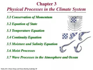
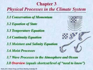
Chapter 3Physical Processes in the Climate System 3.1 Conservation of Momentum 3.2 Equation of State 3.3 Temperature Equation 3.4 Continuity Equation 3.5 Moisture and Salinity Equation 3.6 Moist Processes 3.7 Wave Processes in the Atmosphere and Ocean 3.8 Overview (equals shortcut/level of “need to know”) Neelin, 2011. Climate Change and Climate Modeling, Cambridge UP
Includes equations that are budgets for these conservation laws, and discussion of main balances. Why: Climate models are based on these equations and relationships We can use the main balances to understand features of current climate, El Niño, global warming,.. Know: What we do with the balances & concepts (not equation details) Example (from Section 3.8 of text): Preview of “Section 3.1 Overview” An approximate balance between the Coriolis force and the pressure gradient force holds for winds and currents in many applications (geostrophic balance) (Fig. 3.4). Will come in handy for El Niño … Neelin, 2011. Climate Change and Climate Modeling, Cambridge UP
F a = m d velocity = Coriolis+PGF+gravity+Fdrageqs. 3.4 & 3.5 dt 3.1 Conservation of Momentum F - Force m - Mass a - Acceleration Newton: ma = F (Eq. 3.1) Use force per unit mass for atm/oc. • Acceleration a = rate of change of velocity • Coriolis force: due to rotation of earth (apparent force). • PGF:pressure gradient force. Tends to move air from high to low pressure. • Fdrag: friction-like forces due to turbulent or surface drag. • gravity g = 9.8 m/s2. Neelin, 2011. Climate Change and Climate Modeling, Cambridge UP
Figure 3.1 Schematic of directions and velocities Coordinate system for directions and velocities. Blown up region shows local Cartesian coordinate system (for each region of the sphere). Distances east, north & up are x, y, z. (Also lat, lon j, l) Velocity components u, v, w(eastward, northward, up). Neelin, 2011. Climate Change and Climate Modeling, Cambridge UP
Figure 3.2 Schematic of the Coriolis force • Apparent force that acts on moving masses in a rotating reference frame (Earth rotates once per day) • a leading effect in atm/ocean motions (time scales > day, little friction) Neelin, 2011. Climate Change and Climate Modeling, Cambridge UP
Coriolis force animation Neelin, 2011. Climate Change and Climate Modeling, Cambridge UP
Coriolis force (cont.) • Turns a body or air/water parcel to the right in the northern hemisphere; to the left in the southern hemisphere. • Exactly on the equator, the horizontal component of the Coriolis force is zero • Acts only for bodies moving relative to the surface of the Earth’s equator and is proportional to velocity. • Constant of proportionality is f =(4/1day)sin(latitude), known as the Coriolisparameter; f is positive in the northern hemisphere, negative in the southern hemisphere, and zero at the equator. • [northward force -fu (to right of eastward wind component).] • [eastward force fv (to right of northward wind component).] • [vertical component of Coriolis <<gravity so less important] Neelin, 2011. Climate Change and Climate Modeling, Cambridge UP
df dy Coriolis force (cont.) “Beta effect” change of Coriolis force with latitude • is proportional to cos(latitude) • Always positive and maximum at the equator • matters because Coriolis so important Neelin, 2011. Climate Change and Climate Modeling, Cambridge UP
Figure 3.3 Pressure Gradient Force: e.g., pressure p decreasing eastward ¶p ¶x [Pressure: force per unit area. Change dp across distance dx gives force per volume. High to low, so –dp/ dx . Divide by density r (mass per volume) to get force per mass.] Neelin, 2011. Climate Change and Climate Modeling, Cambridge UP
1 1 ¶p _ ¶x ¶p _ ¶y Pressure Gradient Force, PGF • Force per unit mass, tends to accelerate air from higher to lower pressure • x direction • y direction ¶p ¶x • partial derivatives: pressure change eastward and northward, respectively • density r (mass per unit volume) Neelin, 2011. Climate Change and Climate Modeling, Cambridge UP
d dt velocity = Coriolis+PGF+gravity+FdragEq. 3.2 du dv 1 1 ¶p ¶p _ + Fdrag + Fdrag y x = fv ¶x ¶y dt dt _ _ = fu Horizontal momentum equations (Horizontal = perpendicular to gravity) x-direction (east) Eq. 3.4 y-direction (north) Eq. 3.5 Largest terms (usually) Note: PGF depends on what’s happening to either side; neighboring regions affect each other Neelin, 2011. Climate Change and Climate Modeling, Cambridge UP
1 1 ¶p ¶p ¶x ¶y _ fug = fvg = Figure 3.4 Schematic of geostrophic wind and wind with frictional effects Geostrophic balance: At large scales at mid-latitudes and approaching the tropics the Coriolis force and the pressure gradient force are the dominant forces Neelin, 2011. Climate Change and Climate Modeling, Cambridge UP
_ = g dp dz Pressure-height relation: Hydrostatic balance Eq. 3.8 • Comes from vertical momentum equation but dominated* by balance between vertical pressure gradient and gravity • Pressure at each level in atmosphere or ocean is given by g times amount of mass above it [p=òz¥g dz] *except in small scale features (thunderstorms, squall lines, etc.) Neelin, 2011. Climate Change and Climate Modeling, Cambridge UP
Section 3.1 Overview An approximate balance between the Coriolis force and the pressure gradient force holds for winds and currents in many applications (geostrophic balance) (Fig. 3.4). The Coriolis force tends to turn a flow to the right of its motion in the Northern Hemisphere (left in the Southern Hemisphere); the pressure gradient force acts from high toward low pressure. The Coriolis parameterf varies with latitude (zero at the equator, increasing to the north, negative to the south); this is called the beta-effect ( = rate of change of f with latitude). In the vertical direction, the pressure gradient forcebalancesgravity (hydrostatic balance). This allows us to use pressure as a vertical coordinate. Pressure is proportional to the mass above in the atmospheric or oceanic column. Neelin, 2011. Climate Change and Climate Modeling, Cambridge UP
p = RT 3.2 Equation of State • Relates density to temperature T, pressure p(+other factors) • For the atmosphere: Ideal gas law Eq. 3.10 • density decreases with temperature, incr. with pressure • Ideal gas constant R = 287 J kg-1 K-1, T in Kelvin • For the ocean: • density an empirical function of T, p, and SalinityS • For small T changes can use coeff. of thermal expansion eT (percent density decrease per C of T increase), i.e. • r-r0= -r0 e T(T-T0), • with eT =2.7´10-4C-1 for refc temp T0=22C Neelin, 2011. Climate Change and Climate Modeling, Cambridge UP
Figure 3.5 Application: thermal circulation • UCLA (sea breeze) SM Bay Tropics (Hadley circ) subtropics • West Pacific (Walker circ.) East Pacific • relatively low pressure (at given height) at low levels in warm region; PGF toward warm region (near surface) e.g.: Neelin, 2011. Climate Change and Climate Modeling, Cambridge UP
hydrostatic + ideal gas law gives: • fixed mass per area between pressure surfaces • Warm air less dense greater column thickness (height difference) between two pressure surfaces • p1 below z1 in warm region, so p at z1 is L rel to cool region Neelin, 2011. Climate Change and Climate Modeling, Cambridge UP
dh h Application: sea level rise by thermal expansion • mass of ocean: area*rh.If mass & area constant, while density decreases byd, depth h must change bydh -rdh = hd Eq. 3.16 • recall coeff. of thermal expansion eT (percent density decrease per C of T increase), with eT =2.7*10-4C-1 near 22C: • dr = -reTdT, so • = eTdT • E.g. 300m upper ocean layer warming 3C • dh = 300 ´2.7´10-4C-1 ´ 3C = 0.24m Eq. 3.17 Neelin, 2011. Climate Change and Climate Modeling, Cambridge UP
Section 3.2 Overview Atmos: relationship of density to pressure and temperature from ideal gas law Ocean: density depends on temperature (warmer= less dense, e.g. sea level rise by warming)& salinity (saltier= more dense). Thermal circulations (Fig. 3.5): warm atmospheric column has low pressure near the surface and high pressure aloft relative to pressure at same height in a neighboring cold region. Reason: see Fig. 3.5 PGF near surface toward warm region; Coriolis force may affect circulation but warm region tends to have convergence & rising. e.g.: Walker, Hadley circulations Neelin, 2011. Climate Change and Climate Modeling, Cambridge UP
dT dT dt dt r cw H = Fnet-Fnet sfc bot 3.3 Temperature Equation heat capacity´change of T with time* = heating cw Ocean: = Q Eq. 3.18 cw - heat capacity of waterQ – heatingJ/(kg s)4200 Joule/(kg K) heating related to net flux Fnet in Wm-2: [integrate over layer (´densityr), e.g. surface layer of depthH difference in fluxes (surface minus bottom) Eq. 3.19 ] *dT/dt following “parcel” of water Neelin, 2011. Climate Change and Climate Modeling, Cambridge UP
dT dp 1 _ cp = Q dt dt dp _ top ∫ top sfc QIR FIR FIR = g sfc 3.3 Temperature Equation cp - heat capacityof air at constant p.Q - heating Atmosphere: Eq. 3.20 -work of expanding parcel as p decreases Similar but new term: As in chpt 2:Q = QSolar+ QIR+ Qconvection+ Qmixing Eq. 3.21 Heating integrated over the column: difference in fluxes (top of atm. minus sfc.), [e.g.: Eq. 3.22] Neelin, 2011. Climate Change and Climate Modeling, Cambridge UP
_ dT 1 dt dp dt 3.3.3 Dry Adiabatic lapse rate 0 Adiabatic: no heating cp = Q Eq. 3.20 • Term due to work of expansion important to convection: T decreases as parcel rises (in height) since p decreases • T decreases even though no exchange of heat with environment (negligible loss or gain, since parcel rises fast) • T decrease with height (“lapse rate”) 10 C/km for adiabatic rising/sinking (no condensation: “dry adiabatic”) Neelin, 2011. Climate Change and Climate Modeling, Cambridge UP
Figure 3.6 Thermals Example of rising convective parcel without cloud • Many parcels moving with dry adiabatic lapse rate [10C/km] • Mixing surrounding air (“environment”) is brought to approx same lapse rate* *Why you can ski in the morning and surf in the afternoon Neelin, 2011. Climate Change and Climate Modeling, Cambridge UP
dT dt dT dT dt dt Time derivative following the parcel • Where are transports? Hidden in [along with much complexity] Total derivative: following an air parcel as it moves • For local change of T at fixed location, expand to show transports by wind Neelin, 2011. Climate Change and Climate Modeling, Cambridge UP
∂T = ∂t ∂T ∂t dT ∂T ∂T ∂T ∂T ∂T ∂T + u +v + w dt ∂x ∂x ∂y ∂y ∂z ∂z u +v + w dT dt ∂T ∂T –u = ∂t ∂x Time derivative following the parcel (cont.) Eq. 3.27 Local time derivative at fixed place “Advection” terms: carry properties from one region to another e.g. wind from west uand = 0 (temp of air parcel constant), then the local temp change is given by : …cold air to west gives local temperature dropping Neelin, 2011. Climate Change and Climate Modeling, Cambridge UP
Figure 3.7 Initially simple air parcels being deformed in wind fields • Initially simple patterns become complex [these then feedback on wind field] • Yields chaotic motions • Slight changes in initial conditions yield large changes later Neelin, 2011. Climate Change and Climate Modeling, Cambridge UP
Section 3.3 Overview • Ocean: time rate of change of temperature of water parcel given by heating • for a surface layer: net surface heat flux from the atm. minus the flux out the bottom by mixing • Atmosphere:Temperature eqn. similar to ocean but… • when an air parcel rises, temperature decreases as parcel expands towards lower pressure. • Quickly rising air parcel (e.g. in thermals): little heat is exchanged • temperature decreases at 10 C/km (the dry adiabatic lapse rate). Neelin, 2011. Climate Change and Climate Modeling, Cambridge UP
Section 3.3 Overview (cont.) • Time derivatives following parcel hide complexity of the system : the parcels themselves tend to deform in complex ways if followed for a long time. • Results in the loss of predictability for weather. • The time derivative for temperature at a fixed point is obtained by expanding the time derivative for the parcel in terms of velocity times the gradients of temperature (advection). • Similar procedure applies in other equations. Neelin, 2011. Climate Change and Climate Modeling, Cambridge UP
3.4 Continuity equation Diverging motions Figure 3.7 3-D divergence e.g., ocean sfc. • Conservation of mass: mass = density • volume • Divergence in 3 dimensions D3D rate of change of volume would tend to reduce density • Ocean case: hard to change density much • Horizontal divergence balanced by vertical motions } Neelin, 2011. Climate Change and Climate Modeling, Cambridge UP
= -D3D ∂v ∂u d ∂y ∂x dt D = + 3.4 Continuity equation ] [Details: full eqn. Eq. 3.28 3.4.1 Oceanic continuity equation Horizontal divergence: Eq. 3.30 ∂w Eq. 3.29 D = - Ocean approx. ∂z • Horizontal divergence balanced by net inflow in vertical Neelin, 2011. Climate Change and Climate Modeling, Cambridge UP
∂ ∂p _ D = 3.4.2 Atmospheric continuity equation • Atmospheric continuity eqn.: simple in pressure coord. • recall pressure surfaces are mass surfaces • Horizontal divergence D along pressure surfaces must be balanced by vertical motion [ Eq. 3.31 • vertical velocity in pressure coord.] • e.g., low level convergence balanced by rising motion • [Note pressure increases downward so is negative for rising motions] Neelin, 2011. Climate Change and Climate Modeling, Cambridge UP
drag fu ≈ Fy _ ∂w D = ∂z Coastal upwelling: e.g., Peru; northward wind component along a north-south coast • Drag of wind stress tends to accelerate currents northward • Coriolis force turns current to left in S. Hem • [momentum eqn. ] • u away from coast horizontal divergence upwelling from below[thru bottom of surface layer ≈ 50m] • [Continuity eqn. ] Figure 3.9 Neelin, 2011. Climate Change and Climate Modeling, Cambridge UP
Figure 3.10 Processes leading to equatorial upwelling • Wind stress accelerates currents westward • [wind speed fast relative to currents, so frictional drag at surface slows the wind but accelerates the currents] • Just north of Equator small Coriolis force turns current slightly to right (south of Equator to the left) Þ divergence in surface layer Þ balanced by upwelling from below Neelin, 2011. Climate Change and Climate Modeling, Cambridge UP
Supplementary Fig.: 1998 Annual Ocean Color (Chlorophyll est.) NASA/Goddard Space Flight Center and ORBIMAGE, SeaWiFS Project • In tropics, high biological productivity in equatorial cold tongue and coastal regions due to upwelling of nutrients Neelin, 2011. Climate Change and Climate Modeling, Cambridge UP
∂h ^ + HD = 0 ∂t 3.4.5 Conservation of warm water mass in idealized layer above thermocline Figure 3.11 warm less dense cold dense • Warm light water above thermocline at depth h • Horizontal divergence/convergence in upper layer movement of thermocline [approx. H = mean thermocline depth, D = vertical avg. thru layer ] ^ Neelin, 2011. Climate Change and Climate Modeling, Cambridge UP
Section 3.4 Overview • Conservation of mass can be expressed as horizontal divergence or convergence (of currents or winds) being balanced by changes in the vertical motion. In the atmosphere this holds in pressure coordinates. • Equatorial upwelling results from divergence of ocean surfacecurrents away from the equator. Water must rise from below to compensate. The divergence at the equator occurs due to effects of easterly winds and the Coriolis force (see Figure 3.10). • For the layer of warm water above the thermocline, convergence of upper ocean currents* implies a deepening of the thermocline (see Figure 3.11). *Note upper ocean layer above thermocline typically deeper than surface layer in tropics; equatorial upwelling can occur even while thermocline deepens Neelin, 2011. Climate Change and Climate Modeling, Cambridge UP
dq dt mass of salt Salinity, s = total mass water 3.5 Conservation of mass applied to moisture Moisture and Salinity Equations • conservation of mass: water vapor in atm, salt + water in ocean Sources - Sinks = mass water vapor Specific humidity, q = total mass air • Similarly, for snow models, ice sheets, land hydrology keep track of water mass per unit area • Sink from one can be a source for another: e.g., precipitation is a sink of water substance from the atmosphere, but a source term at the surface of the ocean & land surface; vice versa for evaporation Neelin, 2011. Climate Change and Climate Modeling, Cambridge UP
Links with energy budget: • Keep track of mass of water vapor, liquid water, snow/ice separately because of latent heat • Latent heat of condensation 2.50´106 J kg-1; • Latent heat of of freezing 3.34´105 J kg-1 3.5.3 Application: surface melting on an ice sheet Suppose (during melting season) surface temperature for a region on an ice sheet remains at freezing so additional increment of downward heat flux assoc. with global warming, say 5 W m−2, is used for melting. Rate of decrease of ice thickness = 5 W m−2 (Lfρi)−1 (365 day/yr × 86400 s/day) ≈ 0.5m/yr. So roughly millennial scale to melt 1.5 km where density of ice, ρi = 0.9 × 10³ kg m−2 Neelin, 2011. Climate Change and Climate Modeling, Cambridge UP
Section 3.5 Overview • Conservation of mass gives equations for water vapor (atmosphere) and salinity (ocean). • The main sinks of water vapor are due to moist convection (resulting in precipitation) which at the same time produces convective heating in the temperature equation (from condensation in clouds). The main source of water vapor is evaporation at the surface (it is then transported, mixed, etc). These processes involve small scale motions and must be parameterized. • Salinity at the ocean surface is increased by evaporation and decreased by precipitation. Neelin, 2011. Climate Change and Climate Modeling, Cambridge UP
3.6 Moist Processes Figure 3.12 • At saturation: equilibrium of water vapor with liquid water; • molecules evaporating = molecules condensing • Unsaturated air tends to conserve water vapor concentration • Saturation value increases with temperature, so can saturate by reducing T. Above saturation condensation occurs. Neelin, 2011. Climate Change and Climate Modeling, Cambridge UP
actual water vapor* Relative humidity = saturation value* Figure 3.12 100% 85% 65% [*in units of vapor pressure: converts to specific humidity using total air pressure] Neelin, 2011. Climate Change and Climate Modeling, Cambridge UP
3.6.2 Saturation in convection; lifting condensation level Recall dry adiabat has no heat exchange but T drops with height due to expansion Figure 3.13 (lower part) cloud base • Parcel conserves moisture Þ saturates when T gets cold enough [lifting condensation level = cloud base] • As rises further, condensation occurs Neelin, 2011. Climate Change and Climate Modeling, Cambridge UP
3.6.3 The moist adiabat and lapse rate in convective regions Figure 3.13 • As saturated parcel continues to rise: • Decrease in p decrease in T • more water vapor condenses • T drops less than for unsaturated parcel (roughly 6 C/km as opposed to 10 C/km) • Process still adiabatic [parcel not exchanging heat with environment]: moist adiabatic process Neelin, 2011. Climate Change and Climate Modeling, Cambridge UP
Figure 3.13 (cont.) • If cold parcel rising along “moist adiabat” is warmer than surrounding air it continues to rise [until it reaches level where it is no longer bouyant] • Rising parcels warm troposphere through deep layer [to temperature close to moist adiabat]: T set by warm moist surface air Neelin, 2011. Climate Change and Climate Modeling, Cambridge UP
Section 3.6 Overview • Saturation of moist air depends on temperature according to Figure 3.12. Relative humidity gives the water vapor relative to the saturation value. • A rising parcel in moist convection decreases in temperate according to the dry adiabatic lapse rate until it saturates, then has a smaller moist adiabatic lapse rate. The temperature curve in Figure 3.13 (the moist adiabat) depends on only the surface temperature and humidity where the parcel started. • If this curve is warmer than the temperature at upper levels, convection typically occurs. Neelin, 2011. Climate Change and Climate Modeling, Cambridge UP
3.7 Wave Processes in the Atmosphere and Ocean: Overview • Waves play an important role in communicating effects from one part of the atmosphere to another. • Rossby waves depend on the beta-effect [change of coriolis force with latitude]. Their inherent phase speed is westward. In a westerly mean flow, stationary Rossby waves can occur in which the eastward motion of the flow balances the westward propagation. Stationary perturbations, such as convective heating anomalies during El Nino, tend to excite wavetrains of stationary Rossby waves. Neelin, 2011. Climate Change and Climate Modeling, Cambridge UP
Figure 3.14 Rossby wave westward propagation (mean wind is zero) [If Coriolisparam. f were const., low pressure region could be stationary; winds circulating in balance with PGF] [Increasing f northward (N. Hem.) implies imbalance in mass transport, yields progagation] Neelin, 2011. Climate Change and Climate Modeling, Cambridge UP
Figure 3.15 Typical Rossby wave pattern excited by a stationary source Neelin, 2011. Climate Change and Climate Modeling, Cambridge UP