Download
1 / 52
520 likes | 721 Vues
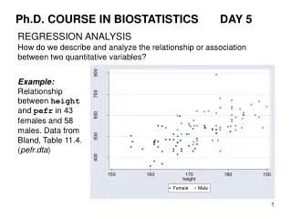
Ph.D. COURSE IN BIOSTATISTICS DAY 5. REGRESSION ANALYSIS How do we describe and analyze the relationship or association between two quantitative variables?. Example: Relationship between height and pefr in 43 females and 58 males. Data from Bland, Table 11.4. ( pefr.dta ).

E N D
Ph.D. COURSE IN BIOSTATISTICS DAY 5 REGRESSION ANALYSIS How do we describe and analyze the relationship or association between two quantitative variables? Example: Relationship between height and pefr in 43 females and 58 males. Data from Bland, Table 11.4. (pefr.dta)
This type of data arises in two situations: Situation 1: The data are a random sample of pairs of observations.In the example: both pefr and height are measured (observed) quantities, i.e. random variables, and none of these variables are controlled by the investigator. Situation 2: One of the variables is controlled by the investigator, and the other is subject to random variation, e.g. in a dose-response experiment, the dose is usually controlled by the investigator and the response is the measured quantity (random variable). Purpose in both cases: To describe how the response (pefr) varies with the explanatory variable (height). Note: A regression analysis is not symmetric in the two variables. Terminology: x= independent/explanatory variable = dose y = dependent/response variable sex = grouping variable
Linear relationship In the mathematical sense the most simple relationship between y and x is a straight line, i.e. Example: does the descriptiondepend on sex? Statistical model In the statistical sense this corresponds to the model: whereE represents the random variation around the straight line. • Random variation • The random variation reflects several sources of variation: • measurement error, (2) biological (inter-individual) variation • and (3) deviations in the relationship from a straight line. • In a linear regression analysis the cumulative contributions from • these sources are described as independent ”error” from a normal distribution .
Statistical model The data consists of pair of observations and the statistical model takes the form: Example: does the parameters depend on sex? where the Ei’s (or equivalently the yi’s) are independent. Unknown parameters The model has 3 unknown parameters: Estimation A linear regression can be performed by most statistical software and spreadsheets. The estimates of aand bare obtained by the method of least squares by minimizing the residual sum of squares: Solution:
Regression for each group Only females shown • In Stata the command is: • regress pefr height if sex==1 -> sex = Female Source| SS df MS Number of obs = 43 --------+---------------------------- F( 1, 41) = 5.65 -Model| 12251.4221 1 12251.4221 Prob > F = 0.0222 Residual| 88856.2222 41 2167.22493 R-squared = 0.1212 --------+---------------------------- Adj R-squared = 0.0997 Total| 101107.644 42 2407.32487 Root MSE = 46.553 -------------------------------------------------------------------- pefr| Coef. Std. Err. t P>|t| [95% Conf. Interval] --------+----------------------------------------------------------- height| 2.912188 1.224836 2.38 0.022 .4385803 5.385795 _cons| -9.170501 203.3699 -0.05 0.964 -419.8843 401.5433 -------------------------------------------------------------------- Note: Estimated regression line: The line pass through with slope
The sampling distribution of the estimates: But note: are not independent estimates p-value for slope = 0 -------------------------------------------------------------------- pefr| Coef. Std. Err. t P>|t| [95% Conf. Interval] --------+----------------------------------------------------------- height| 2.912188 1.224836 2.38 0.022 .4385803 5.385795 _cons| -9.170501 203.3699 -0.05 0.964 -419.8843 401.5433 -------------------------------------------------------------------- p-value for intercept = 0 t-tests of the hypotheses slope = 0 (top) and intercept = 0 (bottom) Confidence intervals for the parameters
Test and confidence intervals Stata gives a t-test of the hypothesis and a t-test of the hypothesis . The test statistics are computed as and These test statistics have a t-distribution with n – 2 degrees of freedom, if the corresponding hypothesis is true. The standard errors of the estimates are obtained from the sampling distribution by replacing the population variance by the estimate . 95% confidence intervals for the parameters are derived as in lecture 2, e.g. as where is the upper 97.5 percentile in a t-distribution with n – 2 degrees of freedom. After the regress command other hypothesized values of the parameters can be assessed directly by ( 1) height = 2.5 F( 1, 41) = 0.11 Prob > F = 0.7382 test height = 2.5 Note: F = t2
Interpretation of the parameters Intercept (): the expected pefr when height = 0, which makes no biological sense. For this reason the reference point on the x-axis is sometimes changed to a more meaningful value, e.g. Physical unit of intercept: as y, i.e. as pefr (litre/minute). Slope (β): the expected difference in pefr between two (female) students A and B, where A is 1 cm taller than B. Physical units of slope: as , i.e. as pefr/height (litre/minute/cm) Standard deviation (σ): The standard deviation of the random variation around the regression line. Approximately 2/3 of the data points are within one standard deviation from the line. The estimate is often called root mean square error. Physical unit of standard deviation: as y, i.e. as pefr (litre/minute). Change of units: If height in the example is measure in meter the slope becomes: (litre/minute/meter)
Residual The residual is the difference between the observed value and the fitted value: Fitted value For the ith observation the fitted value (expected value) is
Checking the model assumptions • Look at the scatter plot of y against x. The model assumes a linear trend. • 2. If the model is correct the residuals have mean zero and approximately constant variance. Plot the residuals (r) against the fitted values ( ) or the explanatory variable x. The plot must not show any systematic structure and the residuals must have approximately constant variation around zero. • 3. The residuals represent estimated errors. Use a histogram and/or a Q-Q plot to check if the distribution is approximately normal. Note: A Q-Q plot of the observed outcomes, the yi’s, can not be used to check the assumption of normality, since the yi’s do not follow the same normal distribution (the mean depends on xi). The explanatory variable, the xi’s, is not required to follow a normal distribution.
Stata: predicted values and residuals are obtained using two predict commands after the regress command: regress pefr height predict yhat, xb(yhat is the name of a new variable) predict res, residuals(res is the name of a new variable) Plots for females Both plots look OK!
Example: Non linear regression Note: The non-linear relationship between y and x is most easily seen from the plot of the residuals against x.
Example: Variance heterogeneity Note: Again, the fact that the variance increase with x is most easily seen from the plot of the residuals against x.
Regression models can serve several purposes: • Description of a relationship between two variables • Calibration • Confounder control and related problems, e.g. to describe the relationship between two variables after adjusting for one or several other variables. • Prediction Re 1. In the example about pefr and height we found a linear relationship and the regression analysis identified the parameters of the ”best” line as Re 2. Example: much modern laboratory measurement equipment do not measure the concentrations in your samples directly, but uses build-in regression techniques to calibrate the measurements against known standards. Re 3. Example: Describe the relationship between birth weight and smoking habit when adjusting for parity and gestational age. This is a regression problem with multiple explanatory variables (multiple linear regression or analysis of covariance)
Example (test of no effect modification): In the data on pefr and height we may want to compare the relationship for males with that for females, i.e. assess if the sex is an effect-modifier of this relationship. The hypothesis of no effect modification is , i.e. that the two regression lines are parallel. A simple test of this hypothesis can be derived from the estimates of the two separate regression analyses. We have an approximately standard normal test statistic is Inserting the values gives z =-0.608, i.e. p-value = 0.543. The slopes does not seem to be different.
Re 4. Example: Predicting the expected outcome for a specified x-value, e.g. predicting pefr for a female with height=175 cm: Stata: lincom _cons+height*175 ( 1) 175 height + _cons = 0 --------------------------------------------------------------- pefr | Coef. Std. Err. t P>|t| [95% Conf. Interval] ------+-------------------------------------------------------- (1) | 500.4623 13.1765 37.98 0.000 473.8518 527.0728 --------------------------------------------------------------- • The t-test assess the hypothesis that pefr= 0 for a 175 cm high female!!! • (nonsense in this case). • To test the hypothesis that pefr is e.g. 400, write • lincom _cons+height*175-400 Note: Prediction using x-values outside the range of observed x-values (extrapolation) should in general be avoided.
DECOMPOSITION OF THE TOTAL VARIATION If we ignore the explanatory variable, the total variation of the response variable y is the adjusted sum of squares (corrected total) When the explanatory variable x is included in the analysis we may ask: How much of the variation in y is explained by the variation in x ? i.e. How large would the variation in pefr be, if the persons have the same height?. residual Deviation: fitted – overall mean Variation about regression = Residual Variation explained by regression = Model
The degrees of freedom are decomposed in a similar way Stata: All this appears in the analysis of variance table in the output from the regress command MS = mean square = SS/df -> sex = Female Source| SS df MS Number of obs = 43 --------+---------------------------- F( 1, 41) = 5.65 Model| 12251.4221 1 12251.4221 Prob > F = 0.0222 Residual| 88856.2222 41 2167.22493 R-squared = 0.1212 --------+---------------------------- Adj R-squared = 0.0997 Total| 101107.644 42 2407.32487 Root MSE = 46.553 The mean squares are two independent variance estimates. If the slope is 0, they both estimate the population variance .
The F-test of the hypothesis: Intuitively, if the ratio is large the model explains a large part of the variation and the slope must therefore differ from zero. This is formalized in the test statistic , which follows an F-distribution (Lecture 2, page 44), if the hypothesis is true. Large values leads to rejection of the hypothesis. Note: Source| SS df MS Number of obs = 43 --------+---------------------------- F( 1, 41) = 5.65 Model| 12251.4221 1 12251.4221 Prob > F = 0.0222 Residual| 88856.2222 41 2167.22493 R-squared = 0.1212 --------+---------------------------- Adj R-squared = 0.0997 Total| 101107.644 42 2407.32487 Root MSE = 46.553 R-squared as a measure of explained variation The total variation is reduced from 101107.644 to 88856.2222, i.e. the reduction is 12.12% or 0.1212 which is found in the right panel as the R-squared value. Adj R-squared is a similar measure of explained variation, but computed from the mean squares. R-squared is also called the ”coefficient of determination”.
THE CORRELATION COEFFICIENT A linear regression describes the relationship between two variables, but not the ”strength” of this relation. The correlation coefficient is a measure of the strength of a linear relation. Example: (fishoil.dta) Fish oil trial (see: day 2, page 11). What is the relationship between the change in diastolic and in systolic blood pressure in the fish oil group?
Use a linear regression analysis? No obvious choice of response. The problem is symmetric. Here the sample correlation coefficient may be a more useful way to summarize the strenght of the linear relationship between the two variables. Pearson’s correlation coefficient Basic properties of the correlation coefficient: symmetric in x and y ifx and y are independent If the observations lie exactly on a straight line with positive/negative slope • Change of origin and/or scale of x and/or y will not change the size of r (the sign is changed if the ordering is reversed)
Stata: • correlate difsys difdia if grp==2 | difsys difdia -------------+------------------ difsys | 1.0000 difdia | 0.5911 1.0000 The correlation is positive indicating a positive linear relationship. The sample correlation coefficient r is an estimate of the population correlation coefficient . A test of the hypothesis is identical to the t-test of the hypothesis . It can be shown that Stata: The command pwcorr difsys difdia,sig gives the correlation coefficient and the p-value of this test. For a linear regression: r2 = R-Squared = Explained variation
Use of correlation coefficients: Correlations are popular, but what do they tell about data? Note: The correlation coefficient only measures thelinear relationship Conclusion: Always make plot of the data!
Misuse of correlation coefficients In general: A correlation should primarily be used to evaluate the association between two variables, when the setting is truly symmetric. The following examples illustrate misuse or rather misinterpretation of correlation coefficients. Comparison of two measurements methods Two studies, each comparing two methods of measuring heights of men. In both studies 10 men were measured twice, once with each method. In such studies a correlation coefficient is often used to quantify the agreement (or disagreement) between the methods. This is a bad idea!
Example 1 Higher correlation in left panel Is a higher correlation evidence of a better agreement ? No, this is wrong!!! A difference vs. average plot reveals that there is a large disagreement between method 1 and 2, see next page.
5.6 cm 0.2 cm Compare the averagedisagreement between the two methods! Note: The correlation coefficient does not give you any information on whether or not the observations are located around the line x = y, i.e. whether or not the methods show any systematic disagreement.
Example 2: Two other studies. The same basic set-up. The plots show: • No systematic disagreement (points are located around the line x = y). • Correlation coefficient in left panel (method 1 vs 2) larger than correlation coefficient in right panel (method 3 vs 4). Better agreement between method 1 and 2 than method 3 and 4 ???
The answer is: No!!! s.d.= 2.8 cm s.d.= 1.6 cm Compare the standard deviations of the differences (Limits of agreement = 2 x s.d., see Lecture 2, p. 29) Note: The correlation is larger between method 1 and 2 because the variation in heights is larger in this study. The correlation coefficient says more about the persons than about the measurement methods!
NON-PARAMETRIC METHODS FOR TWO-SAMPLE PROBLEMS Non-parametric methods, or distribution-free methods, are a class of statistical methods, which do not require a particular parametric form of the population distribution. Advantages: Non-parametric methods are based on fewer and weaker assumptions and can therefore be applied to a wider range of situations. Disadvantages: Non-parametric methods are mainly statistical test. Use of these methods may therefore overemphasize significance testing, which is only a part of a statistical analysis. Non-parametric tests do not depend on the observed values in the sample(s), but only the on the ordering or ranking. The non-parametric methods can therefore also be applied in situations where the outcome is measured on some ordinal scale, e.g. a complication registered as –, +, ++, or +++. A large number of different non-parametric tests has been developed. Here only a few simple test in widespread use will be discussed.
TWO INDEPENDENT SAMPLES: WILCOXON-MANN-WHITNEY RANK SUM TEST Illustration of the basic idea • Consider a small experiment with 5 observations from two groups • Active treatment • Control Hypothesis of interest: the same distribution in the two samples, i.e. no effect of active treatment. For data values 15, 26, 14, 31, 21 (in arbitrary order) there are 120 (=5!) different ways to allocate these five values to . Each allocation is characterized by the ordering of the units. Each ordering is equally likely if the hypothesis is true. An ordering is determined by the ranks of the observations. If e.g. then
Basic idea: Compute sum of rank in treatment group. If this sum is large or small the hypothesis is not supported by the data. There are different combinations of ranks for the observations in the treatment group. Under the hypothesis each of these is equally likely (i.e. has probability 0.10). observed configuration We have p-value = 4·0.1=0.4 Note: The distribution is symmetric. observed value
General case Data: Two samples of independent observations Group 1 from a population with distribution function Group 2 from a population with distribution function Let denote the total number of observations. Hypothesis: The x’s and the y’s are observations from the same (continuous) distribution, i.e. . The alternatives of special interest: the y’s are shifted upwards (or downwards). Test statistic (Wilcoxon’s ranksum test) Sum of ranks in group 1, or Sum of ranks in group 2 A two-sided test will reject the hypothesis for large or small values of . Note: The two test statistics are equivalent since
Some properties of the test statistic If the hypothesis is true, the distribution of the test statistic is completely specified. In particular; the distribution is symmetric and we have Moreover, mean and the variance are given by The formula for the variance is only valid if all observations are distinct. If the data contain tied observations, i.e. observations taking the same value, then Midranks, computed as the average value of the relevant ranks, are used. The variance is then smaller and a correction is necessary. The general variance formula becomes where number of identical observations in the i’th set of tied values
Finding the p-value The exact distribution of the of rank sum statistic under the hypothesis is rather complicated, but is tabulated for small sample sizes, see e.g. Armitage, Berry & Matthews, Table A7 or Altman, Table B10. Note: These tables are appropriate for untied data only. The p-value will be too large if the tables are used for tied data. For larger sample size (e.g. N > 30) the distribution of the rank sum statistic is usually approximated by a normal approximation with the same mean and variance, i.e. the test statistic is approximately a standard normal variate if the hypothesis is true. Some programs (and textbooks) use a continuity correction, and the test statistics then becomes
Rank-sum test with Stata Example. In the Lectures day 2 we used a t-test to compare the change in diastolic blood pressure in pregnant women who were allocated to either supplementary fish oil or a control group. The analogous non- parametric test is computed by the command use fishoil.dta ranksum difdia , by(grp) Two-sample Wilcoxon rank-sum (Mann-Whitney) test grp | obs rank sum expected -------------+--------------------------------- control | 213 44953 45901.5 fish oil | 217 47712 46763.5 -------------+--------------------------------- combined | 430 92665 92665 unadjusted variance 1660104.25 adjustment for ties -3237.25 ---------- adjusted variance 1656867.00 Ho: difdia(grp==control) = difdia(grp==fish oil) z = -0.737 Prob > |z| = 0.4612 Stata computes the approximate standard normal variate without a continuity correction two-sided p-value
The rank-sum test can also be used to analyse a 2×C table with ordered categories. In Lecture 4 (page 42) first parity births in skejby-cohort.dta were cross-classified according to mother’s smoking habits and year of births. To evaluate if the prevalence of smoking has changed we use a rank-sum test to compare the distribution on birth year among smokers and non-smokers. ranksum year if parity==0 , by(mtobacco) gives mtobacco | obs rank sum expected -------------+--------------------------------- smoker | 1311 3473225 3527901 nonsmoker | 4070 11007046 10952370 -------------+--------------------------------- combined | 5381 14480271 14480271 unadjusted variance 2.393e+09 adjustment for ties -2.669e+08 ---------- adjusted variance 2.126e+09 Ho: year(mtobacco==smoker) = year(mtobacco==nonsmoker) z = -1.186 Prob > |z| = 0.2357
Mann-Whitney’s U test Some statistical program packages compute a closely related test statistic, Mann-Whitney’s U test. This test is equivalent to the Wilcoxon rank-sum test, but is derived by a different argument. Basic idea: Consider all pairs of observations (x,y) with one observation from each sample. Let number of pairs with x < y number of pairs with y < x A pair with x = y is counted as ½ in both sums. Extreme values of these test statistics suggest the hypothesis is not supported by the data. One may show that The distributions of these test statistics are therefore a simple translation of the distribution of the rank-sum and the samep-value is obtained.
General comments on the rank-sum test For comparison of two independent samples the rank-sum test is a robust alterative to the t-test. For detecting a shift in location the rank-sum test is never much less sensitive than the t-test, but may be much better if the distribution is far from a normal distribution. The rank-sum test is not well suited for comparison of two populations, which differ in spread, but have essentially the same mean. Non-parametric methods are primarily statistical test. For the shift in location situation, i.e. when is distributed as , where is the unknown shift we may estimate the shift parameter as the median of the differences between one observation from each sample, and a confidence interval for the shift parameter can then be obtained from the rank-sum test. This procedure is not included in Stata. Note: A monotonic transformation of the data, e.g. by a logarithm has no impact on the value of the rank-sum statistic.
TWO PAIRED SAMPLES: WILCOXON’S SIGNED RANK-SUM TEST Basic problem: Analysis of paired data without assuming normality of the variation. Data: A sample of n pairs of observations. Question: Does the distribution of the x’s differ from the distribution of the y’s? Preliminary model considerations: For a pair of observation we may write where and represent the expected response of x and y, and where and are error terms. Assume: Error terms from different pairs are independent and follow the same distribution.
If the error terms and follow the same distribution then the difference has a symmetric distribution with median (and mean) . Statistical model: The n differences are regarded as a random sample from a symmetric distribution F with median . Estimation: The population median is estimated by the sample median. Hypothesis: The x’s and the y’s have the same distribution, or equivalently The sign test A simple test statistic is based on the signs of the differences. If the median is 0, positive and negative difference should be equally likely, and the number of positive differences therefore follows a binomial distribution with p = 0.5. If some differences are zero the sample size is reduced accordingly. Stata:signtest hgoral=craft
Wilcoxon’s signed rank sum test The sign test utilizes only the sign of the differences, not their magnitude. A more powerful test is available is both sign and size of the differences are taken into account. Basic idea: Sort the differences in ascending order of their absolute value (i.e. ignoring the sing of the differences). Use the sum of the ranks of the positive differences as the test statistic. Wilcoxon’s signed rank-sum test sum of ranks of positive differences, when differences are are ranked in ascending order according to absolute value. Alternatively, , defined analogously, can be used. The two test statistics are equivalent. Basic properties: With no ties and zeros present in the sample of differences, the test statistic has a symmetric distribution and
Ties and zeroes among differences Mid ranks are used if some of the differences have the same absolute value, i.e. these differences are given the average value of the ranks that would otherwise apply. Differences that are equal to zero are not included in any of the test statistics. A formula for the variance corrected for ties and zeroes exists and is used by Stata. Zeroes are usually accounted for by ignoring these differences and reducing the sample size according. Finding the p-value The exact distribution of the of Wilcoxon’s signed rank-sum test under the hypothesis is tabulated for small sample sizes (n ≤ 25), see e.g. Armitage, Berry & Matthews, Table A6 or Altman, Table B9. Note: These tables are appropriate for untied data only. The p-value will be too large if the tables are used for data with ties.
Normal approximation For larger sample size (n > 25 ) the distribution of the test statistic is approximated by a normal approximation with the same mean and variance, i.e. the test statistic is approximately a standard normal variate if the hypothesis is true. Stata computes this test statistic using a variance estimate that allows for ties and zeroes. Some programs (and textbooks) use a continuity correction, and the test statistics then becomes The continuity correction has little or no effect even for moderate sample sizes and can safely be ignored.
Wilcoxon’s signed rank-sum test with Stata • Example. In the lectures day 3 we used a paired t-test to compare • counts of T4 and T8 cells in blood from 20 individuals. The analogous • non-parametric test is computed by the command • use tcounts.dta • signrank t4=t8 Wilcoxon signed-rank test sign | obs sum ranks expected -------------+--------------------------------- positive | 12 147 105 negative | 8 63 105 zero | 0 0 0 -------------+--------------------------------- all | 20 210 210 unadjusted variance 717.50 adjustment for ties 0.00 adjustment for zeros 0.00 ---------- adjusted variance 717.50 Ho: t4 = t8 z = 1.568 Prob > |z| = 0.1169 No correction since these data have no ties or zeroes The p-value is larger than 0.05, so the difference between the distribution of T4 and T8 cells is not statistically significant
Example continued Diagnostic plots of these data (day 3, page 31 and 38) suggest that the counts initially should be log-transformed. Note: Transformations of the basic data, the x’s and the y’s, may change the value of Wilcoxon’s signed rank-sum test. • signrank logt4=logt8 sign | obs sum ranks expected -------------+--------------------------------- positive | 12 150 105 negative | 8 60 105 zero | 0 0 0 -------------+--------------------------------- all | 20 210 210 unadjusted variance 717.50 adjustment for ties 0.00 adjustment for zeros 0.00 ---------- adjusted variance 717.50 Ho: logt4 = logt8 z = 1.680 Prob > |z| = 0.0930 Note: the number of positive ranks are unchanged, but the sum of these ranks has changed. The p-value has also changed (a little).
NON-PARAMETRIC CORRELATION COEFFICIENTS Non-parametric correlation coefficients measure the strength of the association between continuous variables or between ordered categorical variables. Spearman’s rho Data: A sample of n pairs of observations. Procedure: Rank the x’s and the y’s, and let Then Spearman’s rho is defined as the usual correlation coefficient computed from the ranks, i.e. We have . If Y increase with X then is positive, if Y decrease with X then is negative.
If X and Yare independent and the data have no tied observations then From Spearman’s rho a non-parametric test of independence between X and Y can be derived. The exact distribution of Spearman’s rho under the hypothesis of independence is complicated, but has been tabulated for small sample sizes, see e.g. Altman, Table B8. Usually the p-value is found by computing the test statistic which approximately has a t-distribution with n – 2 degrees of freedom. Stata’s command spearman uses this approach to compute the p-value, see below.
Kendall’s tau A pair of pairs of observations are called concordant if and or if and , i.e. when the two pairs are ordered in the same way according to X and according to Y. Similarly, a pair of pairs are called discordant if the ordering according to Y is a reversal of the ordering according to X. Let C = number of concordant pairs in the sample D = number of discordant pairs in the sample Ties are handled by adding ½ to both C and D. Then number of pairs of pairs in the sample Let then Kendall’s tau (or tau-a) is defined as Kendall’s tau-b uses a slightly different denominator to allow for ties.
Properties of Kendall’s tau We have . When X and Y are independent and no ties are present in the data it can be shown that Formulas valid for tied data are complicated. Also from Kendall’s tau a non-parametric test of independence between X and Y can be derived. The test statistic is usually based on a normal approximation to S, the numerator of Kendall’s tau. A continuity correction is routinely applied. Stata’s command ktau uses this approach to compute the p-value, see below. Note: Both Spearman’s rho and Kendall’s tau are unchanged if one or both of the series of observations are transformed.
Non-parametric correlation coefficients with Stata • Example. • Consider the data with counts of T4 and T8 cells in blood from 20 persons, • but this time we want to describe the association between the two counts. • spearman t4 t8 Number of obs = 20 Spearman's rho = 0.6511 Test of Ho: t4 and t8 are independent Prob > |t| = 0.0019 The hypothesis of independence is rejected in both cases. Persons with a high T4 value typically also have a high T8 value. • ktau t4 t8 Number of obs = 20 Kendall's tau-a = 0.5053 Kendall's tau-b = 0.5053 Kendall's score = 96 SE of score = 30.822 Test of Ho: t4 and t8 are independent Prob > |z| = 0.0021 (continuity corrected) S = C – D Note: The hypothesis of independence differs from the hypothesis tested with a paired two-sample test