Download
1 / 57
580 likes | 758 Vues
Ph.D. COURSE IN BIOSTATISTICS DAY 1. Interpretation of evidence is an important part of medical research. Evidence is often in the form of numerical data . Statistics : Methods for collection, analysis and evaluation of data. Statistics Descriptive statistics

E N D
Ph.D. COURSE IN BIOSTATISTICS DAY 1 Interpretation of evidence is an important part of medical research. Evidence is often in the form of numerical data. Statistics: Methods for collection, analysis and evaluation of data • Statistics • Descriptive statistics • Tables and plots that highlights important aspects of the data. • Inferential statistics • Analysis and evaluation of evidence in the form of numerical • data. The purpose of the statistical analysis is to extract relevant • information about a (scientific) problem and to draw conclusions • about a population from a sample of individuals. Statistics also include aspects of the design of experiments and observational studies
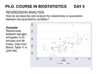
A simple example In Denmark the number of live births per year has varied considerably over the last 20-30 years
In the same period the percentage of boys has been very stable. From 1974 to 2002 the percentage of boys varied between 51.1% and 51.7% with an average of 51.34%
In smaller communities the percentage of boys varied much more. Often the number of girls exceeded the number of boys: Does these data suggest that the percentage of boys born in Odder differs from the national figure? Is the variation from year to year larger than what is expected?
The number of births in Odder varied between 180 and 256 in the period with an average of 224. 95% 75% 50% 25% 5% The lines show so-called 5, 25, 50, 75 and 95-percentiles of the distribution of a proportion based on a sample of size 224 when the true proportion is 51.3%
For a (random) sample of size 224 statistical theory predicts that • 50% of the proportions fall above the full line and 50% below • 50% of the proportions fall between the two dashed lines • 90% of the proportions fall between the two dotted lines We cannot expect to get exactly these percentages in every sample. Statistical methods allows us to describe the data and evaluate if the observations are consistent with the expectations. In this example: information about the total population is known, so we were able to describe the variation in the samples from these results. Usually: No data on population level. Instead one or several samples are available. The population may be rather unspecific, e.g. ”similar patients” Typical problems: compare samples, describe associations
Basic components of a statistical analysis • Specification of a statistical model. • The model gives a formal description of the systematic differences • and the randomness in the data • Estimation of population characteristics. • These are often parameters of the statistical model • Validation of the statistical model. • The relevance of the statistical analysis depends on the validity • of the assumptions • Testing hypotheses about the model parameters. • The hypotheses reflects the (scientific) questions that led to • the data collection
Statistics – some key aspects • Common sense • Inductive inference • Study of variation • Methods for data reduction • Models • Quantification of uncertainty • Mathematics • Computer programs • Inductive inference • Methods for drawing conclusion about a population of individuals • from a sample of specific individuals • Variation • Biological data are usually subject to large variation: • Which aspects of the variation in the data represent systematic differences? • Which aspects of the variation in the data are random fluctuations?
Variation (continued) • Studies are often carried out to assess the size of systematic effects • or to correct for some (known) systematic effects when evaluating • the size of other sytematic effects. • Many sources of random variation, e.g. • Measurement error • Biological variation: Intra- and inter-individual variation • Observer variation • Data reduction • How do we describe a large data set with a few relevant numbers • without loosing important information? • Statistical models – Quantification of uncertainty - Mathematics • An idealized probabilistic description of the proces that generates the data. The model includes some parameters which describe systematic and random variation. • The statistical analysis gives estimates of the parameters and limits of uncertaincy for the estimates.
Computer programs • Statistical analyses often involve large amount of computations. • Simple calculations can be done by pocket calculators and spreadsheet, but special-purpose software are usually convenient. • In this course the program Stata version 9 is used for all calculations. • For an short introduction to Stata see the manual • Getting started with Stata – For windows In Stata 9 statistical calculations and plots can be specified either by use of pull-down menus or by use of commands. Menus are especially convenient for beginners and occasional users, but once the basic commands are learned the command language provide a much faster way to interact with the program, and a series of commands can be saved for documentation or later use.
A typical Stata session involves • Starting Stata: Double-click on the Stata icon • Defining a log-file to contain the results • log using “e:\kurser\f2004\outfile.log • log using “e:\kurser\f2004\outfile.log , text • reading the data • use “e:\kurser\f2004\mydata.dta” • a series of commands that perform the desired analyses • saving the results • log close • saving the new data, if data have been modified • save “e:\kurser\f2004\mynewdata.dta • A series of commands can be created and saved in a command file, • mycommand.do, and run in batch mode from within Stata
STATA – basic commands for data manipulation Example 1 The file skejby-cohort.dta contains information on the mother and the newborn for all deliveries in the maternity ward at Skejby Hospital in period 1993-95. • The information in the file is stored in 8 variables. To get the data into Stata and list the first 5 records • cd E:\kurser\f2004\ • log using outfile01.log , text • use skejby-cohort • listin 1/5 +--------------------------------------------------------------------------+ | bweight gestage mtobacco cigarets bsex mage parity date | |--------------------------------------------------------------------------| 1. | 4000 41 . . girl . 0 30793 | 2. | 2640 36 . . girl . 0 141095 | 3. | 3000 39 smoker 10 girl 41 2 60995 | 4. | 3330 41 . . boy 39 2 100694 | 5. | 3700 39 nonsmoker 0 girl 39 1 10495 | +--------------------------------------------------------------------------+
To list only records satisfying a specified condition use • list bweight bsex mage if mage>45 +-----------------------+ | bweight bsex mage | |-----------------------| 1. | 4000 girl . | 2. | 2640 girl . | 1008. | 3745 boy . | 2079. | 3100 boy 46 | +-----------------------+ Note that missing values are included since in Stata a missing value is represented by a (very) large number • Other uses of list • list mage in 1/100 if parity==0 • list if bsex==. , clean compress compact format with no lines • Notesmissing value • A logical “equal to” is written as == • Options are place after a comma. A full list of options are available • in the help-menu: Help→Stata Command…→write name of the • command in field→OK or using the keyboard: Alt-h-o
Generating new variable and changing existing variables New variables are defined using the command generate. Existing variables are changed with the command replace • Example • generate day=int(date/10000) • generate mon=int((date-10000*day)/100) • generate year=1900+date-10000*day-100*mon • generate primi=(parity==0) if parity<. • list day mon year date parity primi in 1/2 , clean Output: day mon year date parity primi 1. 3 7 1993 30793 0 1 2. 14 10 1995 141095 0 1 Variables can be labeled to further explain the contents • label variable day “day of birth” • label variable mon “month of birth” • label variable year “year of birth” • label variable primi “first child”
Labels may also be added to the categories of a categorical variables • label define primilab 0 “multipari” 1 “primipari” • label values primi primilab • list parity primi in 1/2 , clean parity primi 1. 0 primipari 2. 0 primipari Date variables are a special type of variables. Dates are represented as days since January 1 1960, but can easily be shown in a more useful format • generate bdate=mdy(mon,day,year) • list day mon year date bdate in 1 , clean • format bdate %d • list date bdate in 1 , clean number of days since 1.1.1960 day mon year date bdate 1. 3 7 1993 30793 12237 -------- date bdate 1. 30793 03jul1993
New variables can also be defined using the command recode. The variable primi generated above can alternatively be defined as • recode parity (0=1)(.=.)(else=0) , generate(primi) Note: the option generate ensures that the information is placed in a new variable. If omitted the result is placed in the old variable and the original contents is loss. • Adding a column with record numbers to the file • generate recno=_n • Sorting the data according to a variable • sort mage • Renaming and reordering of variables • rename bsex sex • order recno bdate • Any variable not mentioned follows the variables mentioned • A short description of a variable, including labels (if any) and format • describe mage mtobacco
Selection of records and variables • To keep only data on births from 1993 • keep if year==1993 • To drop records for mothers younger than 20 • drop if mage < 20 • To keep variables from bweight to cigarets and parity • keep bweight-cigarets parity • To drop the variables mtobacco and cigarets • drop mtobacco cigarets • To keep 15% random sample of the data in memory • sample 15 • To obtain a random sample of size 200 records (other records • are dropped) • sample 200, count • To recover all data the file must be re-read into memory with use
SUMMARIZING DATA - DESCRIPTIVE STATISTICS • Main data types • Qualitative or categorical data • Quantitative data – two subtypes: discrete and continuous • The data contain information on different, qualitative or quantitative, • aspects of the individuals/objects in the sample. • These aspects are usually called variables • Qualitative variables: Each individual/object falls in a class or category • The categories may be ordered (e.g. low, moderate, high) or unordered • (e.g. boy, girl). In the data file the categories are assigned (arbitrary) • numbers, but labels may be used to clarify the meaning. • Examples of qualitative variables in the file skejby-cohort.dta • bsex “sex of child” • the variable has categories “boy” and “girl” • mtobacco “smoking habits of mother” • the variable has categories “smoker” and “nonsmoker”
The categories of a qualitative variable, their numerical codes and labels can be displayed using the command codebook Example The command codebookbsex gives the following output ------------------------------------------------------------------ bsex sex of child ------------------------------------------------------------------ type: numeric (float) label: sexlab range: [1,2] units: 1 unique values: 2 missing .: 4/12955 tabulation: Freq. Numeric Label 6674 1 boy 6277 2 girl 4 . Frequencies, and relative frequencies of the different categories can also be obtained with the commands tabulate or tab1. Missing values are ignored unless the option missing is added.
Examples • tabu bsex , missing • tabu bsex year , col nofreq nokey • Output • sex of | • child | Freq. Percent Cum. • ------------+----------------------------------- • boy | 6,674 51.52 51.52 • girl | 6,277 48.45 99.97 • . | 4 0.03 100.00 • ------------+----------------------------------- • Total | 12,955 100.00 • sex of | year of birth • child | 1993 1994 1995 | Total • -----------+---------------------------------+---------- • boy | 51.37 51.80 51.43 | 51.53 • girl | 48.63 48.20 48.57 | 48.47 • -----------+---------------------------------+---------- • Total | 100.00 100.00 100.00 | 100.00 • Several other options are also available. Using if and in tabulations • can be restricted to subsets of the data, e.g. • tabu bsex year if mage>35
The tabulations can be displayed as bar charts or pie charts with the • commands, e.g. • graph hbar (count) recno, over(mtobacco) missing • graph bar (count) recno, over(mtobacco) missing • graph pie , over(mtobacco) missing • The option missing includes a category for missing values. • The first command produces the following graph: missing values
Separate plots for each value of another variable may easily be obtained • Example: Plots of the number of births for each months of the year • for each of the years 1993, 1994 and 1995 produced by • graph bar (count) recno , /// • over(mon) by(year) bar(1,bfc(gs5)) bfc= bar filling color gs= gray scale indicate that the command continues on the next line
SUMMARIZING QUANTITATIVE VARIABLES • Quantitative variables contain numerical information. Two types • Discrete variables : only integer values are possible. • Example: parity. • Continuous variables: Measurements can in principle be any number • in a range (due to rounding not all numbers may occur in practice) • Examples: bweight, mage • For quantitative variables a table of frequencies or • relative frequencies is less useful. • When summarizing the values of a quantitative variable focus is • usually on • What is a typical value? • How much variation is there in the data? • For each question several data summaries, so-called statistics, • are available
Typical value Data: a sample of n observations The sample mean is the average of the observations The sample median: the value which separates the smallest 50% from the largest 50% Percentiles (or quantiles) 5-percentile: The value for which 5% of the observations are smaller than this value 10-percentile: The value for which 10% of the observations are smaller than this value etc. 25-percentile is called the lower quartile, 50-percentile is the median, 75-percentile is called the upper quartile The quartiles divide the observations in four groups of the same size.
Describing variation in the data The average deviation from the sample mean is always 0, so this is not a useful measure of the variation in the data. One could instead consider the average absolute deviation from the sample mean, but this number is mathematically less attractive. The average squared deviation is usually preferred Sample variance Sample standard deviation is the square root of the sample variance and is measured in the same units as the observations Range: The largest observation minus the smallest observation Interquartile range: The upper quartile minus the lower quartile
Summarizing quantitative variables with Stata • summarize bweight gestage mage • Output: • Variable | Obs Mean Std. Dev. Min Max • -------------+-------------------------------------------------------- • bweight | 12955 3517.842 584.7701 520 5880 • gestage | 12851 39.52751 1.883722 24 44 • mage | 12952 28.89554 4.828905 15 46 • The option detail gives additionalinformation • summarize bweight , detail • Output: • birth weight • ------------------------------------------------------------- • Percentiles Smallest • 1% 1605 520 • 5% 2580 580 • 10% 2850 600 Obs 12955 • 25% 3200 610 Sum of Wgt. 12955 • 50% 3540 Mean 3517.842 • Largest Std. Dev. 584.7701 • 75% 3900 5620 • 90% 4200 5640 Variance 341956 • 95% 4400 5750 Skewness -.6593171 • 99% 4800 5880 Kurtosis 5.238386
Summary statistics of a quantitative variable for each category of a • qualitative variable • bysort year: summarize bweight • Alternative command for obtaining selected summary statistics • tabstat bweight gestage mage, /// • stat(n mean med p5 p95 sd range iqr) • Output: • stats | bweight gestage mage • ---------+------------------------------ • N | 12955 12851 12952 • mean | 3517.842 39.52751 28.89554 • p50 | 3540 40 29 • p5 | 2580 36 21 • p95 | 4400 42 37 • sd | 584.7701 1.883722 4.828905 • range | 5360 20 31 • iqr | 700 2 6 • ---------------------------------------- • Options include 25 different summary statistics. See help on tabstat • for details. Also a by() option is allowed, e.g. • tabstat bweight , stat(n mean sd)by(bsex)
DISPLAYING QUANTITATIVE DATA - GRAPHS • Useful plots for describing a set of observations include histograms, • cumulative distribution functions and Box-plots. • The command • histogram bweight if year==1993 & gestage==40,freq • gives the following plot
The user may specify options to define the number of categories • – called bins – the starting point and the width of the categories. • Otherwise Stata finds suitable values. • In the plot above Stata chose bin=31, start=2000, width=106.45161 • The command • histogram bweight if year==1993 & gestage==40 , /// • freq start(2000) width(200) • gives the following plot
The option freq gives frequency (counts) on the y-axis. • If omitted the density is shown (i.e. total area=1). • “Uncategorized” data are plotted with the option discrete, e.g. • histogram bweight if year==1993 & gestage==40 , /// • freq discrete Some birth weights are more popular than others!
Interpretation of standard deviations The distribution of birth weight for a given gestational age looks fairly symmetric. For such distributions we have that Approximately 67% of the observations fall in the interval from to Approximately 95% of the observations fall in the interval from to Example The skejby-cohort.dta includes 1477 birth weights in week 40 in 1993. For this sample we have an average birth weight of 3622.7 gram and the standard deviation is 463.0 gram. The interval mean±sd becomes [3159.7,4085.7] and contains 68.9% (1018 out of 1477) observations. The interval mean±2sd becomes [2696.7,4548.7] and contains 95.5% (1411 out of 1477) observations.
For small data sets dot plots provide a useful alternative to histograms, • especially when comparing two or several groups. e.g. • dotplot bweight if gestage==37 , /// • centerover(year) mcolor(black) dots are centered marker color Several additional options are available.
Box plots, also called box-and-whiskers plots, are related to dot plots, but can also be used with larger data sets. Box plots shows quartiles and medians as a box, lines indicate position of data outside the quartiles, and individual outliers are shown. bar line color marker color graph box bweight if gestage==37 , /// over(year) bar(1,blc(black)) m(1,mco(black)) Outliers Upper adjacent value = largest obs. smaller than upper quatile plus 1.5*IQR Upper quartile Median Lower Quartile Defined similarly Note: Several versions are in use – definitions of specific details differ!
The cumulative distribution function shows the cumulative frequencies of the observations i.e. the proportion of observations smaller than or equal to x plotted against x. • cumul bweight if year==1993 & gestage==40 , /// • generate(cdf) equal • line cdf bweight if year==1993 & gestage==40 , /// • sort connect(J) connect points with a step function
Descriptive statistics – from the sample to the population The descriptive methods are mainly useful for an initial phase of the analysis where the purpose is to understand the main features of the data and in the final stages of the analysis where the purpose is to communicate the main findings The statistical summaries of the collected data are usually interpreted as estimates of the similar quantities in the population from which the sample are drawn. The population may be well-defined, e.g. all birth in Denmark in a given year, but often the population is rather vaguely defined, e.g. similar patients treated in the future. Moreover, due to selection, missing values and non-response the population that the sample represents may not be identical to the population for which we want to draw conclusion.
Examples • Assuming that births in Odder in 1995 can be considered as a random sample of births in Denmark (in 1995) the relative frequency, or proportion, of boys observed there is interpreted as an estimate of the probability of a randomly selected (singleton) pregnancy in Denmark results in boy. • For babies born in week 40 and included in the Skejby cohort the 10 percentile of the birth weight distribution was 3070 gram. Thus, the estimated probability of a birth weight under 3070 gram for a baby born in week 40 is 10% (for babies born in Denmark in the mid-90’s). • The average birth weight for children born in week 38 and included in the Skejby cohort is 3274 gram. Thus, the expected birth weight in week 38 is estimated to • 3274 gram (for babies born in Denmark in the mid-90’s).
From relative frequencies to probabilities For categorical variables and discrete variables we used a table to display the relative frequency of each possible outcome in the sample. If the sample size increases to infinity (the sample becomes the total population) these relative frequencies are interpreted as probabilities showing the theoretical distribution of the random variable. The terminology ” a random variable” is used to stress that the values of a variable vary in a random fashion among individuals in a population. The probabilities describe the outcome for a randomly selected individual from the population or the distribution of the random variable. For continuous variables such tables are not feasible since the outcome may take any value in a given range and an infinite number of outcomes are therefore possible. The theoretical distribution is therefore usually described by a cumulative distribution function or a probability density function.
For a random variable X with cumulative distribution function F we have: The value of the cumulative distribution function at a, F(a), describes the probability of an outcome less than or equal to a. Outcome of X is less than or equal to a Example The probability of a value less than 1.5 is equal to 54%
The probability density function, or density function, is the theoretical counterpart of a histogram scaled such that the area under the curve is 1 Relation between density function f and cumulative distribution function F The area under the density function up to a is equal to F(a), the probability that X is less than or equal to a.
Statistics as estimates of population characteristics An estimate is based on a (random) sample from the population and is therefore not necessarily the correct value for the population. However, the commonly used estimates are all unbiased, i.e. they do not differ from the true value in a systematic way. Estimates may, on the other hand, differ from the true value in an unsystematic, random, way. The purpose of a statistical analysis is, among other things, to quantify the uncertainty in the estimates. In a statistical analysis the random variation in the observations are used to derive a description of the random variation in the estimates based on a statistical model, which is an idealized description of the processes that generate the data. Using probability theory the uncertainty in the estimates can be deduced from the random variation in the sample.
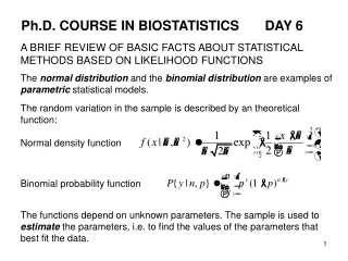
THE BINOMIAL DISTRIBUTION – A SIMPLE EXAMPLE OF A • STATISTICAL MODEL • Consider a series of n experiments, where n is some fixed number. • Assume that • Each experiment has two possible outcomes, usually referred to as “success” and “failure”. • The probability of a “success” is denoted p and is the same in all experiments. • The experiments are mutually independent i.e. knowledge of the outcome of one experiment does not change the probability of a “success” in another experiment. • These assumptions are e.g. fulfilled if we want to study coin tosses. • Here we believe that p=0.5 and there is no need for an experimentally • based estimate. • In other situations the probability of success is unknown and we may • want to derive an estimate of this probability
Intuitively the relative frequency of successes in the n experiments should be used to estimate the probability of a “success”. What is the properties of this estimate? If the binomial assumptions are fulfilled the following result is available: The number of successes follows a binomial distribution, i.e. the probability of getting exactly y successes in n experiments are given by the expression Here and n-y failures and the binomial coefficient gives the number of such sequences of length n. represents the probability of a sequence if y successes The binomial distribution with n=224 and p=0.5134 was used to derive percentiles for the number of boys per year born in Odder (page 5)
The probability function (left) and the cumulative probability function (right) for a binomial distribution with n=224 and p=0.5134 The expected number of successes, to be interpreted as the average number of successes in a large number of identical experiments, is In the example above the expected value is therefore boys out of 224 births.
The variance of the number of successes, i.e. the expected value of the squared deviation from the mean, is and the standard deviation of the number of successes becomes In the example above we have If the ”experiment” was repeated a large number of times we would therefore expect the number of successes to fall in the interval from 100 to 130 approximately 95% of the times, since
The relative frequency (or proportion) is the number of successes divided by the number of experiments, viz. The distribution function of the relative frequency is therefore obtained from the distribution function of y by rescaling the x-axis (divide by n). Moreover Expected value of the proportion Variance and standard error of the proportion Interpretation: The expected value (or mean value), the variance and the standard error are the values of these quantities that one would find in a sample of proportions obtained by repeating the binomial experiment a large number of times and for each experiment compute the proportion.
THE NORMAL DISTRIBUTION The normal, or Gaussian, distribution is the most important theoretical distributions for continuous variables. • Normal distributions: • A class of distributions of the same shape, but with different means and/or variances. • Continuous distributions with sample space (the possible values) equal to all real numbers. A normal distribution is completely determined by its mean and variance. These are called the parameters of the distribution. Notation: mean , variance , X ~ Density function : There is no closed form expression for the cumulative distribution function.
Examples of Normal distributions same mean, but different variances different means, same variance
Relations between normal distributions If X has a normal distribution with mean and variance then has a normal distribution with mean and variance The standardized variable has a standard normal distribution, i.e. a normal distribution with mean 0 and variance 1. The cumulative distribution function and density function for a standard normal distribution are usually denoted and , respectively. Tables of these function are widely available. The density function of a normal distribution is symmetric about the mean.
Selected values of the normal, cumulative distribution function • We see that • The probability of a value in the interval from mean-sd to mean+sd • is approximately 68% • The probability of a value in the interval from mean-2sd to mean+2sd • is approximately 95% • Exactly 95% of the values lies in the central prediction interval:
The use of the normal distribution in statistical analyses Many frequency distributions resemble a normal probability distribution in shape, possibly after a suitable transformation of the data. The name “normal” should not be taken literally to indicate that the distribution represents the normal behavior of random variation. The importance of the normal distribution in statistics lies not so much in its ability to describe a wide range of observed frequency distributions, but in the central place it occupies in sampling theory. In “large” samples the random error associated with parameter estimates and other statistics derived from the observations can usually be approximated very well by a normal distribution. This is a mathematical result which follows from the so-called central limit theorem. Many statistical procedures assumes that the data can be considered as a random sample from a normal distribution. The adequacy of this assumption should always be assessed.