Two Data Sets
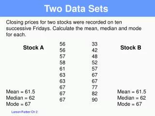
Two Data Sets. Closing prices for two stocks were recorded on ten successive Fridays. Calculate the mean, median and mode for each. 56 33 56 42 57 48 58 52 61 57 63 67

Two Data Sets
E N D
Presentation Transcript
Two Data Sets Closing prices for two stocks were recorded on ten successive Fridays. Calculate the mean, median and mode for each. 56 33 56 42 57 48 58 52 61 57 63 67 63 67 67 77 67 82 67 90 Stock A Stock B Mean = 61.5 Median = 62 Mode = 67 Mean = 61.5 Median = 62 Mode = 67
Measures of Variation Range = Maximum value – Minimum value Range for A = 67 – 56 = $11 Range for B = 90 – 33 = $57 The range is easy to compute but only uses two numbers from a data set.
Measures of Variation To learn to calculate measures of variation that use each and every value in the data set, you first want to know about deviations. The deviation for each value x is the difference between the value of x and the mean of the data set. In a population, the deviation for each value x is: In a sample, the deviation for each value x is:
Deviations Stock A Deviation 56 56 57 58 61 63 63 67 67 67 – 5.5 – 5.5 – 4.5 – 3.5 – 0.5 1.5 1.5 5.5 5.5 5.5 56 – 61.5 56 – 61.5 57 – 61.5 58 – 61.5 The sum of the deviations is always zero.
Population Variance Population Variance: The sum of the squares of the deviations, divided by N. x 56 56 57 58 61 63 63 67 67 67 – 5.5 – 5.5 – 4.5 – 3.5 – 0.5 1.5 1.5 5.5 5.5 5.5 30.25 30.25 20.25 12.25 0.25 2.25 2.25 30.25 30.25 30.25 188.50 Sum of squares
Population Standard Deviation Population Standard Deviation: The square root of the population variance. The population standard deviation is $4.34.
Sample Variance and Standard Deviation To calculate a sample variance divide the sum of squares by n – 1. The sample standard deviation, s, is found by taking the square root of the sample variance.
Summary Population Variance Population Standard Deviation Sample Variance Sample Standard Deviation Range = Maximum value – Minimum value
Data with symmetric bell-shaped distribution have the following characteristics. Empirical Rule (68-95-99.7%) 13.5% 13.5% 2.35% 2.35% –4 –3 –2 –1 0 1 2 3 4 About 68% of the data lies within 1 standard deviation of the mean About 95% of the data lies within 2 standard deviations of the mean About 99.7% of the data lies within 3 standard deviations of the mean
The mean value of homes on a street is $125 thousand with a standard deviation of $5 thousand. The data set has a bell shaped distribution. Estimate the percent of homes between $120 and $135 thousand. Using the Empirical Rule 105 110 115 120 125 130 135 140 145 $120 thousand is 1 standard deviation below the mean and $135 thousand is 2 standard deviations above the mean. 68% + 13.5% = 81.5% So, 81.5% have a value between $120 and $135 thousand.
For any distribution regardless of shape the portion of data lying within k standard deviations (k > 1) of the mean is at least 1 – 1/k2. Chebychev’s Theorem For k = 2, at least 1 – 1/4 = 3/4 or 75% of the data lie within 2 standard deviation of the mean. For k = 3, at least 1 – 1/9 = 8/9 = 88.9% of the data lie within 3 standard deviation of the mean.
Chebychev’s Theorem The mean time in a women’s 400-meter dash is 52.4 seconds with a standard deviation of 2.2 sec. Apply Chebychev’s theorem for k = 2. Mark a number line in standard deviation units. 2 standard deviations A 45.8 48 50.2 52.4 54.6 56.8 59 At least 75% of the women’s 400-meter dash times will fall between 48 and 56.8 seconds.

