Download
1 / 7
90 likes | 454 Vues
Solution of 2D Navier-Stokes equations in velocity-vorticity formulation using FD. Remo Minero Scientific Computing Group – Dep. Mathematics and Computer Science. y. (-1,1). (1,1). D. O. (-1,-1). (1,-1). 2D NAVIER-STOKES EQUATIONS. where D is [-1; 1] x [-1; 1]. x. NUMERICAL METHOD.

E N D
Solution of 2D Navier-Stokes equations in velocity-vorticity formulation using FD Remo Minero Scientific Computing Group – Dep. Mathematics and Computer Science SMARTER meeting
y (-1,1) (1,1) D O (-1,-1) (1,-1) 2D NAVIER-STOKES EQUATIONS where D is [-1; 1] x [-1; 1] x SMARTER meeting
NUMERICAL METHOD • Temporal discretization: • Advection term: Adams-Bashforth scheme • Convection term: Crank Nicolson scheme • 2nd order Runge-Kutta scheme for the 1st time step • Spatial discretization: • Finite differences • Influence matrix technique to enforce boundary condition for 2nd order accuracy Accuracy dependent on derivatives’ discretization (e.g. 1st order for upwind, 2nd for centred differences, etc.) SMARTER meeting
SELF ORGANIZATION OF VORTICES • Random initial condition for u, initial value for follows consistently. (1 – Re=1000 ) (11 – Re=2500 ) SMARTER meeting
Comparing results and performances with already existing codes FUTURE PERSPECTIVES Investigation on time evolution of some physical quantities like E, and L Different initial conditions/ boundary conditions Steep gradient of near the walls: LDC SMARTER meeting
BC Coarse grid Fine grid Defect Max t non to have instabilities t x x x tn+1 tn-1 tn tn+2 LDC IN TRANSIENT PROBLEMS SMARTER meeting
BC Coarse grid Fine grid Defect x x x x x x x x 0 0 L L LDC WITH SPECTRAL METHODS ? SMARTER meeting