Download
1 / 60
600 likes | 725 Vues
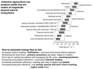
Intensive aquaculture can produce yields that are orders of magnitude beyond natural ecosystems. How to maximize energy flow to fish Increased nutrient loading— fertilization + ammonia and anoxia tolerant species Shortening the food chain— primary consumers (eg carps, tilapia or mullets)

E N D
Intensive aquaculture can produce yields that are orders of magnitude beyond natural ecosystems How to maximize energy flow to fish Increased nutrient loading—fertilization + ammonia and anoxia tolerant species Shortening the food chain—primaryconsumers (eg carps, tilapia or mullets) Don’t rely on natural recruitment and managing the life cycle—stocking/hatcheries Increasing consumption efficiency—small pens intensive feeding Increased assimilation efficiency—feeding with easy to digest food pellets Increased production efficiency—low activity species that don’t mind crowding, , highly turbid water
Many aquaculture proponents argue that aquaculture reduces harvesting pressure on wild fisheries. Salmonid aquaculture not very trophically efficient, food pellets made from by-catch of wild species Major water quality issues—nutrient pollution from cages, anti-fouling paint, antibiotics, habitat destruction Transmit diseases to wild salmonids—bacteria, viruses, protozoans, fungi, “fish lice” –parasitic copepods and other Crustacea Genetic problems when domestic escapees compete with or interbreed with wild fish Lepeophtheirus salmonis Argulus
Rivers support more fish biomass than lakes for the same TP Level? Why? Rivers Fish community biomass kg ● ha-1 Lakes Total Phosphorus µg ● L-1 Log B = 0.94+ 0.52 (± 0.09) Log TP -0.18 (± 0.05) L/R, RMS=0.27, R2=0.71
Zooplankton abundance in reservoirs depends on the physical regime.
Summarizing concepts on Secondary production • The organic matter produced by primary producers (NPP) is used by • a web of consumers • NPP is used directly by primary consumers (herbivores and detritivores), which are in • turn consumed by carnivores. • Measurement of 2o Production is done by estimating the rate of growth of individuals • and multiplying by the number of individuals per unit area in the cohort (age or size group). • The efficiency of secondary production ranges from 5-20% (Avg 10%) • at each trophic level. • Efficiency depends on several factors--palatability, digestibility, energy requirements • for feeding (activity costs)(eg homeotherms vs poikilotherms , other limiting factors • eg water, and nutrient quality of food. • Trophic efficiency can be represented as the product of CE*AE*PE, each of which • is dependent on one or more of the above factors. • The yields of many important fisheries depends on a combination of NPP, the • length ofthe food chain leading to the fish being harvested, and the efficiency • of each step. • Many of the species that we harvest or very high in the food chain, so a great deal • of NPP is required to support them.
Lakes have zonation structured by physical forces such as light, wind and waves. • different zones in the lake had different types of plants and animals
Zones in a river system are less distinct • But they are functionally very important The River Continuum Concept • Physical forces change gradually along a river • Elevation↓ • Slope ↓ • Temperature and nutrients ↑ • Drainage area and discharge ↑ • Width of channel and floodplain ↑ • Mean velocity ↑ • Mean depth ↑ • Turbidity ↑ • Sediments, erosional, alluvial, to depositional • Shading ↓ • Periphyton, macrophytes ↑, then ↓ • Phytoplankton and zooplankton ↑ • Coarse detritus input highest upstream • Fine detritus accumulates downstream • Benthic invertebrate community changes • shredders, grazers, collectors • Fish community changes • Cold water to warm water species http://www.d.umn.edu/~seawww/depth/rivers/art/figure1_4.jpg
Allochthonous input—Detritus processing • Dead plant biomass breaks down slowly and their nutrients can remain tied up in as organic detritus for long periods of time • Primary production in many ecosystems depends more on its recycling rate ie mainly decomposition of plant detritus, than on loading rates • Aquatic plants break down more rapidly than terrestrial plants, and woody plants are very slow to decompose because they contain lignin, which most bacteria and fungi can’t digest.
Leaf processing • Wetting and breadown of cuticle • Leaching of soluble components (DOM) • Colonization by bacteria and fungi • Increase in protein content • Colonization by invertebrates • Enhances microbial action • Breakdown into small fragments
Invertebrate detritiivores find leaves much more to their liking after they have been colonized by bacteria and fungi
Detritus processing in a stream • Shredders enhance microbial action • (bacteria & fungi) • convert CPOM to FPOM • Food for microdetritivores
Processing of FPOM by microdetritivores Shredders-macrodetritivores collectors-microdetritivores Filter-feeders, deposit-feeders
Litter bag experiments have been used to study decomposition of detritus • Nutrient content of the detritus, especially N greatly increases decomposition rate, • as does increased temperature • and mesh size 100 % Weight remaining % 0.5 mm mesh Larger invertebrates get into the litter bags if the mesh is coarse 2 mm mesh 10 20 30 days
The interplay between the autochothonous and the allochtonous food chain Allochthonous input Autochthonous input
The River Discontinuum: Dams and wiers Stream Fragmentation, A wier blocking fish movement a hanging culvert can block fish movement http://www.cee.mtu.edu/~dwatkins/images/aqua3pics/hatchery-weir.jpg http://www.nzfreshwater.org/thumbnails/culvert.jpg
Dams/Reservoirs interrupt the river continuum • create entirely new habitats
Exponential Time
b<m b=m b>m
Density dependent birth and death Per capita birth,death b=b0-b1B m=m0+m1B b0 Slope=b1 m0 Slope=m1 K is called the carrying capacity K Biomass B
per capita rate of increase slows down linearly as the biomass increases and reaches 0 when the carrying capacity (K) is reached. • per capita rate of increase reaches an upper limit of r0 as B approaches 0 • It becomes negative when B>K Is called the logistic equation B K
B K/2 K
B K/2 K
What would happen to a population at K/2 subjected to a harvest rate of C B K/2 K is called the Maximum Sustainable Yield (MSY)
The logistic model * C B K/2 K
An operational example A lake that hasn’t been fished for 20 yr is opened for fishing and annual creel surveys show that CPUE is declining rapidly CPUE Kg/hr • The estimated total catch varies from year to year but the trend rapidly becomes apparent and the lake is closed • After a 9-yr moratorium the population has gradually bounced back, and the fishery is opened again with more restrictive limits Catch Kg/yr • After signs of tapering off limits are tightened even further. Year
How can such a population be managed with the logistic model? We don’t know B, K or r0 We can assume that CPUE is a linear function of Biomass (eg B=q*CPUE Where q is called the “catchability” factor We can also assume that the population is at K to start with CPUE Kg/hr Catch Kg/yr Year
The catch (C) in the first year was 1020 kg, at the rate of 1.0 kg/fisherman hr. • The following year the CPUE went down to 0.9 kg/fisherman hr. • Assuming that the population was at its K, and that the CPUE reflects the biomass linearly, B=q *CPUE, then dB/dt at K will be 0, and the entire catch will be subtracted from the biomass present. • That is we assume that there will be no significant recruitment or growth response to compensate for thinning within the first season • The response to the first year’s thinning will be reflected in the next year’s catch data • assume the change in CPUE reflects the change in B, • (D CPUE)/CPUE = (D B)/B, 0.1/1=1000/K. Therefore K =10,000 kg • And CPUE =q B, that is 1.0 kg/hr =q * 10,000 kg, • so q =1kg/hr/10000 kg = 0.0001kg/hr/kg • The next year the catch rises to 1050 kg, and the CPUE falls to 0.83 kg/hr. This catch appears to be unsustainable at this B level, but how much would have been sustainable?
The next year the catch rises to 1050 kg, and the CPUE falls to 0.83 kg/hr. • This catch appears to be unsustainable at this B level, but how much would have been sustainable? • Using the catchability estimate q we can translate the drop in CPUE and estimate that the biomass dropped from 9000 to 8300 kg (a drop of 700), and reason that if a catch of 1050 caused a drop of 700, then a catch of 350 would have been sustainable at that level of biomass. • We can then repeat this for every year, including the years where the fishery is closed • CPUE can still be estimated from catch and release fishing if the fishery is closed. • In this way each year’s catch combined with the change that takes place in CPUE the following year can allow you to estimate the sustainable catch for that year
Actual catches in kg/yr Estimates of sustainable catch By comparing the catch for each year to the change in biomass (estimated from change in CPUE) we can estimate the catch that would have been sustainable each year For the first 10 yr catches were unsustainably high and the population crashed, After the new limits were put in they tended to oscillate around the estimated catch. Catch Kg/yr CPUE Kg/hr
Fit to the logistic curve from the lake time series dB/dt MSY (r0K)/4=990 K/2 = 5000 Biomass If (r0K)/4 = 990 kg/yr and K=10000 kg, then r0=0.39 kg*kg-1yr-1
Suppose we have a lake with a population of 10,000 kg of pike where fishing has not been allowed for at least 20 years. Fishing is then opened up for several years and the population is knocked back to 5,000 kg. Assume that growth follows the logistic curve. (a) What would the biomass be after 10 yr if r0 were 0.2 kg/kg/yr (b) If after closure it recovers to 9,800 kg in 10 years. Find r0?
(c) What should be the maximum sustainable yield of this fishery? (d) If the population were reduced to 2,000 kg, would a quota of 500 kg/yr be sustainable?, 1000kg?
Suppose we have a lake with a population of 10,000 kg of pike where fishing has not been allowed for at least 20 years. Fishing is then opened up for several years and the population is knocked back to 5,000 kg. Assume that growth follows the logistic curve. Over what range of biomass would a yield of 600 kg/yr be sustainable without causing a reduction in biomass?
Constant Quota fishing at levels approaching the MSY shortens the biomass range the population will recover, and the likelihood of entering the danger zone increases. Once the danger zone is entered fishing must stop or be severely curtailed Danger zone Stable biomass range Catch rate B K/2 K Maximum Sustainable Yield (MSY)
The red zone is much bigger if the curve is strongly skewed right
What if we consider a fishery based on constant effort rather than constant quota The catch isn’t as great but the likelihood of entering the red zone is lower Catch = qB Slope=q Stable range C B K/2 K
Foodweb relationships between fish predators and prey • Bottom up • Richer systems have higher productivity at all trophic levels • Enrichment usually increases the biomass of the top trophic level in the web. • Top down • Predators usually reduce the biomass of their prey • And cause changes in the structure of prey communities • Lake Michigan example
Bottom-up Fish biomass dependent on nutrient loading Reductions in fish biomass usually accompany reductions in nutrient loading
Intensive aquaculture can produce yields that are orders of magnitude beyond natural ecosystems How to maximize energy flow to fish Increased nutrient loading—fertilization + ammonia and anoxia tolerant species Shortening the food chain—primaryconsumers (eg carps, tilapia or mullets) Don’t rely on natural recruitment and managing the life cycle--stocking Increasing consumption efficiency—small pens intensive feeding Increased assimilation efficiency—feeding with easy to digest food pellets Increased production efficiency—low activity species, highly turbid water