First analysis steps
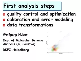
First analysis steps. o quality control and optimization o calibration and error modeling o data transformations Wolfgang Huber Dep. of Molecular Genome Analysis (A. Poustka) DKFZ Heidelberg. Acknowledgements. Anja von Heydebreck Günther Sawitzki


First analysis steps
E N D
Presentation Transcript
First analysis steps o quality control and optimizationo calibration and error modelingo data transformations Wolfgang Huber Dep. of Molecular Genome Analysis (A. Poustka) DKFZ Heidelberg
Acknowledgements Anja von Heydebreck Günther Sawitzki Holger Sültmann, Andreas Buness, Markus Ruschhaupt, Klaus Steiner, Jörg Schneider, Katharina Finis, Stephanie Süß, Anke Schroth, Friederike Wilmer, Judith Boer, Martin Vingron, Annemarie Poustka Sandrine Dudoit, Robert Gentleman, Rafael Irizarry and Yee Hwa Yang: Bioconductor short course, summer 2002 and many others
a microarray slide Slide: 25x75 mm 4 x 4 or 8x4 sectors 17...38 rows and columns per sector ca. 4600…46000 probes/array Spot-to-spot: ca. 150-350 mm sector: corresponds to one print-tip
Terminology sample: RNA (cDNA) hybridized to the array, aka target, mobile substrate. probe: DNA spotted on the array, aka spot, immobile substrate. sector: rectangular matrix of spots printed using the same print-tip (or pin), aka print-tip-group plate: set of 384 (768) spots printed with DNA from the same microtitre plate of clones slide,array channel: data from one color (Cy3 = cyanine 3 = green, Cy5 = cyanine 5 = red). batch: collection of microarrays with the same probe layout.
Image Analysis Raw data • scanner signal • resolution: • 5 or 10 mm spatial, • 16 bit (65536) dynamical per channel • ca. 30-50 pixels per probe (60 mm spot size) • 40 MB per array spot intensities 2 numbers per probe (~100-300 kB) … auxiliaries: background, area, std dev, …
R and G for each spot on the array. Image analysis 1. Addressing. Estimate location of spot centers. 2. Segmentation. Classify pixels as foreground (signal) or background. • 3. Information extraction. For • each spot on the array and each • dye • foreground intensities; • background intensities; • quality measures.
Segmentation adaptive segmentation seeded region growing fixed circle segmentation Spots may vary in size and shape.
spot intensity data n one-color arrays (Affymetrix, nylon) two-color spotted arrays Probes (genes) conditions (samples)
log-ratio Which genes are differentially transcribed? same-same tumor-normal
3000 3000 x3 ? 1500 200 1000 0 ? x1.5 A A B B C C But what if the gene is “off” (below detection limit) in one condition? ratios and fold changes Fold changes are useful to describe continuous changes in expression
ratios and fold changes • Many interesting genes will be off in some of the conditions of interest • If you want expression measure (“net normalized spot intensity”) to be an unbiased estimator of abundance • many values 0 • need something more than (log)ratio • 2. If you let expression measure be biased • can keep ratios. • how do you chose the bias?
Raw data are not mRNA concentrations The problem is less that these steps are ‘not perfect’; it is that they may vary from gene to gene, array to array, experiment to experiment.
Systematic Stochastic o similar effect on many measurements o corrections can be estimated from data o too random to be ex-plicitely accounted for o “noise” Calibration Error model Sources of variation amount of RNA in the biopsy efficiencies of -RNA extraction -reverse transcription -labeling -photodetection PCR yield DNA quality spotting efficiency, spot size cross-/unspecific hybridization stray signal
bi per-sample normalization factor bk sequence-wise probe efficiency hik ~ N(0,s22) “multiplicative noise” ai per-sample offset eik ~ N(0, bi2s12) “additive noise” modeling ansatz measured intensity = offset + gain true abundance
“multiplicative” noise “additive” noise The two-component model raw scale log scale B. Durbin, D. Rocke, JCB 2001
Calibration ("normalization") Correct for systematic variations. To do: fit appropriate "correction parameters" ai, bi (and possibly more…) and apply to the data. "Heteroskedasticity"(unequal variances) weighted regression or variance stabilizing transformation Outliers: use a robust method
data (cDNA slide): relation between mean u=E(Yik) and variance v=Var(Yik): the variance-mean dependence
variance stabilization Xu a family of random variables with EXu=u, VarXu=v(u). Define var f(Xu ) independent of u derivation: linear approximation
variance stabilization f(x) x
1.) constant variance 2.) const. coeff. of variation 3.) offset 4.) microarray variance stabilizing transformations
the arsinh transformation - - - log u ——— arsinh((u+uo)/c)
parameter estimation o maximum likelihood estimator: straightforward – but sensitive to deviations from normality o model holds for genes that are unchanged; differentially transcribed genes act as outliers. o robust variant of ML estimator, à la Least Trimmed Sum of Squares regression. o works as long as <50% of genes are differentially transcribed
Least trimmed sum of squares regression minimize - least sum of squares - least trimmed sum of squares
evaluation: effects of different data transformations difference red-green rank(average)
Coefficient of variation cDNA slide: H. Sueltmann
evaluation: a benchmark for Affymetrix genechip expression measures o Data: Spike-in series: from Affymetrix 59 x HGU95A, 16 genes, 14 concentrations, complex background Dilution series: from GeneLogic 60 x HGU95Av2, liver & CNS cRNA in different proportions and amounts o Benchmark: 15 quality measures regarding -reproducibility -sensitivity -specificity Put together by Rafael Irizarry (Johns Hopkins) http://affycomp.biostat.jhsph.edu
good affycomp results (28 Sep 2003) bad
Summary log-ratio 'glog' (generalized log-ratio) - interpretation as "fold change" + interpretation even in cases where genes are off in some conditions + visualization + can use standard statistical methods (hypothesis testing, ANOVA, clustering, classification…) without the worries about low-level variability that are often warranted on the log-scale
Availability oimplementation in R oopen source package vsn on www.bioconductor.org oBioconductor is an international collaboration on open source software for bioinformatics and statistical omics
PCR plates Scatterplot, colored by PCR-plate Two RZPD Unigene II filters (cDNA nylon membranes)
print-tip effects F(q) q (log-ratio)
spotting pin quality decline after delivery of 5x10⁵ spots after delivery of 3x10⁵ spots H. Sueltmann DKFZ/MGA
spatial effects R Rb R-Rbcolor scale by rank another array: print-tip color scale ~ log(G) color scale ~ rank(G) spotted cDNA arrays, Stanford-type
Batches: array to array differences dij = madk(hik -hjk) arrays i=1…63; roughly sorted by time
Density representation of the scatterplot (76,000 clones, RZPD Unigene-II filters)
Affymetrix files Main software from Affymetrix: MAS - MicroArray Suite. DAT file: Image file, ~10^7 pixels, ~50 MB. CEL file: probe intensities, ~400000 numbers CDF file: Chip Description File. Describes which probes go in which probe sets (genes, gene fragments, ESTs).
Image analysis DAT image files CEL files Each probe cell: 10x10 pixels. Gridding: estimate location of probe cell centers. Signal: • Remove outer 36 pixels 8x8 pixels. • The probe cell signal, PM or MM, is the 75th percentile of the 8x8 pixel values. Background: Average of the lowest 2% probe cells is taken as the background value and subtracted. Compute also quality values.
Data and notation PMijg , MMijg= Intensities for perfect match and mismatch probe j for gene g in chip i i = 1,…, n one to hundreds of chips j = 1,…, J usually 11 or 16 probe pairs g= 1,…, G 6…30,000 probe sets. Tasks: calibrate (normalize) the measurements from different chips (samples) summarize for each probe set the probe level data, i.e., 16 PM and MM pairs, into a single expression measure. compare between chips (samples) for detecting differential expression.
expression measures: MAS 4.0 Affymetrix GeneChip MAS 4.0 software uses AvDiff, a trimmed mean: o sort dj = PMj -MMj o exclude highest and lowest value o J := those pairs within 3 standard deviations of the average
Expression measures MAS 5.0 Instead of MM, use "repaired" version CT CT= MM if MM<PM = PM / "typical log-ratio" if MM>=PM "Signal" = Tukey.Biweight (log(PM-CT)) (… median) Tukey Biweight: B(x) = (1 – (x/c)^2)^2 if |x|<c, 0 otherwise
Expression measures: Li & Wong dChip fits a model for each gene where • qi: expression index for gene i • fj: probe sensitivity Maximum likelihood estimate of MBEI is used as expression measure of the gene in chip i. Need at least 10 or 20 chips. Current version works with PMs only.
Affymetrix: IPM = IMM + Ispecific ? log(PM/MM) From: R. Irizarry et al., Biostatistics 2002 0
position- and sequence-specific effects wi(s): Naef et al., Phys Rev E 68 (2003) Chemistry wi i
Expression measures RMA: Irizarry et al. (2002) o Estimate one global background value b=mode(MM). No probe-specific background! o Assume: PM = strue + b Estimate s0 from PM and b as a conditional expectation E[strue|PM, b]. o Use log2(s). o Nonparametric nonlinear calibration ('quantile normalization') across a set of chips.