Download
1 / 20
200 likes | 274 Vues
Learn to compute range and standard deviation for grouped and ungrouped data, interpret standard deviation significance, and analyze data variability. Master variance, sample standard deviation, and calculate dispersion measures effectively.

E N D
Learning Objectives for Section 11.3 Measures of Dispersion • The student will be able to compute the range of a set of data. • The student will be able to compute the standard deviation for both grouped and ungrouped data. • The student will be able to interpret the significance of standard deviation. Barnett/Ziegler/Byleen Finite Mathematics 11e
11.3 Measures of Dispersion In this section, you will study measures of variability of data. In addition to being able to find measures of central tendency for data, it is also necessary to determine how “spread out” the data is. Two measures of variability of data are the range and the standard deviation. Barnett/Ziegler/Byleen Finite Mathematics 11e
Measures of Variation • Example 1. Heights (in inches) of 5 starting players from two basketball teams: A: 72 , 73, 76, 76, 78 B: 67, 72, 76, 76, 84 • Verify that the two teams have the same mean heights, the same median and the same mode. Barnett/Ziegler/Byleen Finite Mathematics 11e
Range • To describe the difference in the two data sets, we use a descriptive measure that indicates the amount of spread or variablility or dispersion in a data set. • Definition: the range is the difference between maximum and minimum values of the data set. • Example 1 (continued) • Range of team A: 78-72=6 • Range of team B: 84-67=17 • Advantage of range: it is easy to compute • Disadvantage: only two values are considered. Barnett/Ziegler/Byleen Finite Mathematics 11e
Sample Standard Deviation • Unlike the range, the sample standard deviation takes into account all data values. The following procedure is used to find the sample standard deviation. • Step 1. Find the mean of data. Example, Team A: Barnett/Ziegler/Byleen Finite Mathematics 11e
Sample Standard Deviation(continued) • Step 2. Find the deviation of each score from the mean • Note that the sum of the deviations is zero: Barnett/Ziegler/Byleen Finite Mathematics 11e
Sample Standard Deviation(continued) • Step 3. Square each deviation from the mean. Find the sum of the squared deviations. Barnett/Ziegler/Byleen Finite Mathematics 11e
Sample Variance • Step 4. The sample variance is determined by dividing the sum of the squared deviations by (n-1) (number of scores minus one) Example: For Team A, the sample variance is Barnett/Ziegler/Byleen Finite Mathematics 11e
Step 5. The standard deviation is the square root of the variance. The mathematical formula for the sample standard deviation isExample: the sample standard deviation for Team A is Sample Standard Deviation Barnett/Ziegler/Byleen Finite Mathematics 11e
Procedure to Calculate Sample Standard Deviation 1. Find the mean of the data. 2. Set up a table with 3 columns which lists the data in the left hand column and the deviations from the mean in the next column. 3. In the third column, square each deviation and then find the sum of the squares of the deviations. 4. Divide the sum of the squared deviations by (n-1). 5. Take the positive square root of the result. Barnett/Ziegler/Byleen Finite Mathematics 11e
Example • Find the sample variance and standard deviation of the data5, 8, 9, 7, 6 (by hand) Barnett/Ziegler/Byleen Finite Mathematics 11e
Example • Find the sample variance and standard deviation of the data5, 8, 9, 7, 6 (by hand) • Answer: Variance is approximately 2.496. Standard deviation is approximately 1.581. Barnett/Ziegler/Byleen Finite Mathematics 11e
Standard Deviation for Grouped Data 1. Find each class midpoint xi and compute the mean. 2. Find the deviation of each class midpoint from the mean 3. Each deviation is squared and then multiplied by the class frequency. 4. Find the sum of these values and divide the result by (n-1) (one less than the total number of observations). 5. Take the square root. Barnett/Ziegler/Byleen Finite Mathematics 11e
Example of Standard Deviation for Grouped Data This frequency distribution represents the number of rounds of golf played by a group of golfers. Mean is 2201.5/75=29.3533. Barnett/Ziegler/Byleen Finite Mathematics 11e
Example (continued) = 8.37579094 Barnett/Ziegler/Byleen Finite Mathematics 11e
Interpreting the Standard Deviation • The more variation in a data set, the greater the standard deviation. • The larger the standard deviation, the more “spread” in the shape of the histogram representing the data. • Standard deviation is used for quality control in business and industry. If there is too much variation in the manufacturing of a certain product, the process is out of control and adjustments to the machinery must be made to insure more uniformity in the production process. Barnett/Ziegler/Byleen Finite Mathematics 11e
Empirical Rule • If a data set is “mound-shaped” or “bell-shaped”, then • approximately 68% of the data lies within one standard deviation of the mean • about 95% of the data lies within two standard deviations of the mean. • about 99.7 % of the data falls within three standard deviations of the mean. • This means that “almost all” the data will lie within 3 standard deviations of the mean, that is, in the interval determined by Barnett/Ziegler/Byleen Finite Mathematics 11e
Empirical Rule (continued) • Yellow region is 68% of the total area. This includes all data within one standard deviation of the mean. • Yellow region plus brown regions include 95% of the total area. This includes all data that are within two standard deviations from the mean. Barnett/Ziegler/Byleen Finite Mathematics 11e
Example of Empirical Rule The shape of the distribution of IQ scores is a mound shape with a mean of 100 and a standard deviation of 15. A) What proportion of individuals have IQ’s ranging from 85 – 115? B) between 70 and 130? C) between 55 and 145? Barnett/Ziegler/Byleen Finite Mathematics 11e
Example of Empirical Rule The shape of the distribution of IQ scores is a mound shape with a mean of 100 and a standard deviation of 15. A) What proportion of individuals have IQ’s ranging from 85 – 115? (about 68%) B) between 70 and 130? (about 95%) C) between 55 and 145? (about 99.7%) Barnett/Ziegler/Byleen Finite Mathematics 11e