1. Hana ChocklerAlexander IvriiArie MatsliahShiri MoranZiv Nevo IBM Research - Haifa Incremental formal verification of hardware

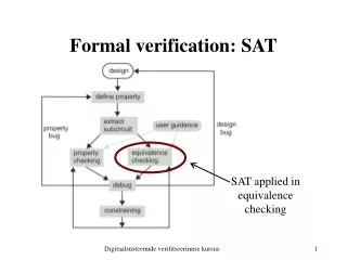
2. Formal verification (hardware) • Effective, but computationally expensive • In many scenarios, similar verification tasks are performed repetitively: • Regression verification • Update to design • Update to specifications • Coverage verification • Can we store and reuse information to reduce amount of redundant computation? Design Spec Verification tool Pass / Fail

3. Incremental formal verification safety properties hardware extract relevant part of previously saved information Design Spec DB ic3 Verification tool store reusable information Pass / Fail

4. Outline • inductive proofs and inductive strengthening • saving information • ic3 overview • what is saved? • reusing saved information • extracting relevant parts (w.r.t. new design/spec) • checking if verification can be concluded • injecting into ic3 • conclusion and experimental results

5. FSMs and safety properties All states • x1,x2,…,xn – state variables (latches) • I – initial states • T – transition relation • R – all reachable states • Ri – states reachable within i steps from I • P – (safety) property ┐P R Rk-1 … T(s,t) R2 R1 I

6. Inductive proofs (for R  P) • Simple induction: • I  P, P ^T  P‘ Sufficient butnot necessary. Almost never holds in practice.. • Solution: find G such that: • I  G • G ^ T  G‘ • G  P Gis over-approximation ofR ! All states ┐P G R I

7. All states ┐P G R I ic3 - basic properties • Complete – always terminates with correct result • SAT based, no unrolling • If P is invariant, produces a CNF formula G, s.t.: • I  G • G ^ T G’ • G  P • If not, produces a (generalized) CEX α0, α1,…, αks.t.: • all α0states belong to I • all αistates lead to some αi+1state • αkis in ┐P I … ┐P a0 a1 ak

8. (bounded) inductive invariants in ic3 P Fk-1 Fk F1 Img(Fk-2) Img(Fk-1) … F0=I Img(F0) • Clause sets/CNF formulas F1,...,Fk • Initially: k=1, F1 = P (assume I  P and Img(I)  P) • Invariants: • I  F1 ...  Fk  P (furthermore, for all i, Fi+1is a subset of Fi) • Img(Fi)  Fi+1 • Ri Fi • If Fi = Fi+1for some i<k, then Fiis an inductive strengthening that proves R  P

9. ic3 progress and termination • Inductive clauses that block “bad state predecessors” are added to the sets Fi, in a way that maintains the containment invariants • Once in a while, clauses are “pushed” to higher Fi’s • ic3 terminates when either: • Fi=Fi+1 for some i  we save the inductive invariant Fi • it finds a CEX: chain of bad state predecessors that starts at I  we generalize and save the CEX + we save the absolute invariants * Absolute inductive invariants are those clauses that were “pushed” beyond Fk

10. How to reuse saved invariants? Finding maximal inductive invariant • Input: I, T, P and C = {c1,…,cm} - candidate invariant clauses • Output: PASS or maximum subset Q of C such that I  Q and Q ^ T  Q‘ * Note: if Q1^ T  Q’1and Q2^ T  Q‘2then (Q1 U Q2) ^ T  (Q’1 U Q’2) • Once such Q is found, we can “inject” it into ic3 by conjoining Q with all sets Fi • This saves ic3 the effort of “rediscovering” the invariants from Q

11. Finding Q using a SAT solver * that supports SolveWithAssumptions(a1,...,ak) 1. cnfize T and I, set Q:=C 2. remove from Qall clauses that are not implied by I 3. for every ci in Q, introduce two auxiliary vars: xiand y’i 4. for every i, cnfize xi ci and y’i ┐c’i 5. SolveWithAssumptions(x1, ..., x|Q|, (y’1 v ... v y’|Q|)) 6. if unsat: Q is invariantif sat: remove from Q each ciwith assign(y’i)=1 and goto 5 7. if Q  P outputPASS, ow return Q

12. Overall approach inject maximal inductive-invariant into ic3 Design Spec DB maximal invariant/ CEX extraction Verification tool save inductive invariant / CEX Pass / Fail inductive invariants / generalized CEXes

13. Experimental results(accumulated runtimes in seconds) 758 designs from HWMCC’10 17 IBM designs

14. Concluding remarks • ic3 can be used to save small inductive proofs, and generalized CEXes • the technique is robust since ic3 invariants and CEXes involve only state variables • makes coverageandregressionverification almost immediate • parts from inductive proofs can be used even if design/spec has significantly changed • saved information is reusableeven when verification result changes

15. The End

16. Generalizing assignments • Input: circuit C and assignment a such that C(a)=y • Output: partial assignment a’ such that C(b)=y for all extensions b of a’ * a’ is obtained by subst. some of the 0,1 values in a with x (don’t cares) Standard algs: • start from root and propagate “cares” • start from leaves and propagate “don’t cares”

17. Generalizing assigns. with solver • Input: circuit C and assignment a such that C(a)=y • Output: partial assignment a’ such that C(b)=y for all extensions b of a’ 1. cnfize C 2. SolveWithAssumptions(┐(C(a)=y), a1, ..., an) * must return unsat (BCP) 3. if aiparticipates in the conflict set a’i = ai else set a’i = x

18. Generalizing assigns. with solver 1. cnfize C 2. SolveWithAssumptions(┐(C(a)=y), a1, ..., an) * must return unsat (BCP) 3. if aiparticipates in the conflict set a’i = ai else set a’i = x Advantages: 1. easy to enforce additional constraints (e.g. learnt clauses and invars) 2. can order the variables in the assumptions acc. to some priority 3. can run after standard algs 4. no real solving – just BCP 5. shrinks by additional 30-40% after ternary simulation (like in PDR)