EECS 380: Wireless Communications Weeks 3-4: Propagation
990 likes | 1.43k Vues
EECS 380: Wireless Communications Weeks 3-4: Propagation. Michael L. Honig Department of EECS Northwestern University. October 2009. Why Study Radio Propagation?. To determine coverage Must determine path loss Function of Frequency Distance

EECS 380: Wireless Communications Weeks 3-4: Propagation
E N D
Presentation Transcript
EECS 380: Wireless CommunicationsWeeks 3-4: Propagation Michael L. Honig Department of EECS Northwestern University October 2009
Why Study Radio Propagation? • To determine coverage • Must determine path loss • Function of • Frequency • Distance • Terrain (office building, urban, hilly, rural, etc.) Can we use the same channels? Need “large-scale” models
Why Study Radio Propagation? • To enable robust communications (MODEM design) • How can we guarantee reliable communications? • What data rate can we provide? • Must determine signal statistics: • Probability of outage • Duration of outage Received Power Deep fades may cause an outage time Need “small-scale” models
Will provide answers to… • What are the major causes of attenuation and fading? • Why does the achievable data rate decrease with mobility? • Why are wireless systems evolving to wider bandwidths (spread spectrum and OFDM)? • Why does the accuracy of location tracking methods increase with wider bandwidths?
Propagation Key Words • Large-scale effects • Path-loss exponent • Shadow fading • Small-scale effects • Rayleigh fading • Doppler shift and Doppler spectrum • Coherence time / fast vs slow fading • Narrowband vs wideband signals • Multipath delay spread and coherence bandwidth • Frequency-selective fading and frequency diversity
Propagation Mechanisms:1. Free Space distance d reference distance d0=1 Reference power at reference distance d0 Path loss exponent=2 P0 In dB: Pr = P0 (dB) – 20 log (d) slope = -20 dB per decade Pr (dB) P0 = Gt Gr (/4)2 log (d) 0 wavelength antenna gains
Wavelength • Wavelength >> size of object signal penetrates object. • Wavelength << size of object signal is absorbed and/or reflected by object. • Large-scale effects refers to propagation over distances of many wavelengths.Small-scale effects refers to propagation over a distances of a fraction of a wavelength. (meters) = c (speed of light) / frequency
Dipole Antenna 802.11 dipole antenna cable from transmitter wire (radiator)
Radiation Pattern: Dipole Antenna Dipole axis Dipole axis Electromagnetic wave radiates outfrom the dipole axis. Cross-section of doughnut pattern
Antenna Gain Pattern Red curve shows the antenna gain versus angle relative to an isotropic pattern (perfect circle) in dB. Often referred to as dBi, dB “isotropic”. -5 dB (factor of about 1/3) relative to isotropic pattern Dipole pattern (close to isotropic)
Antenna Gain Pattern Dipole pattern (vertical) 90 degree sector
Path loss ~ 13 dB / 100 meters or 130 dB / 1 km Increases linearly with distance Requires repeaters for long distances Path loss ~ 30 dB for the first meter + 20 dB / decade 70 dB / 100 meters (2 decades) 90 dB / 1 km(3 decades) 130 dB / 100 km! Increases as log (distance) Repeaters are infeasible for satellites Attenuation: Wireless vs. Wired 1 GHz Radio (free space) Unshielded Twisted Pair Short distance Wired has less path loss. Large distance Wireless has less path loss.
Incident E-M wave reflected wave q q Length of boundary >> wavelength l transmitted wave Propagation Mechanisms 2. Reflection 3. Diffraction 4. Scattering Signal loss depends on geometry Hill
Why Use > 500 MHz? • There is more spectrum available above 500 MHz. • Lower frequencies require larger antennas • Antenna dimension is on the order of awavelength = (speed of light/frequency) = 0.6 M @ 500 MHz • Path loss increases with frequency for the first meter • 10’s of GHz: signals are confined locally • More than 60 GHz: attenuation is too large(oxygen absorbs signal)
700 MHz Auction • Broadcast TV channels 52-69 to be relocated in Feb. 2009. • 6 MHz channels occupying 698 – 806 MHz • Different bands were auctioned separately: • “A” and “B” bands: for exclusive use (like cellular bands) • “C” band (11 MHz): must support open handsets, software apps • “D” band (5 MHz): shared with public safety (has priority) • Commenced January 24, 2008, ended in March
Why all the Hubbub? • This band has excellent propagation characteristics for cellular types of services (“beach-front property”). • Carriers must decide on technologies: 3G, LTE, WiMax,… • Rules for spectrum sharing can be redefined…
C Band Debate • Currently service providers in the U.S. do not allow any services, applications, or handsets from unauthorized 3rd party vendors. • Google asked the FCC to stipulate that whoever wins the spectrum must support open applications, open devices, open services, open networks (net neutrality for wireless). • Verizon wants to maintain “walled-garden”. • FCC stipulated open applications and devices, but not open services and networks: spectrum owner must allow devices or applications to connect to the network as long as they do not cause harm to the network • Aggressive build-out requirements: • Significant coverage requirement in four years, which continues to grow throughout the 10-year term of the license.
Sold to… • Verizon • Other winners: AT&T (B block), Qualcomm (B, E blocks) • Total revenue: $19.6 B • $9.6 B from Verizon, $6.6 B from AT&T • Implications for open access, competition?
D Band Rules • Winner gets to use both D band and adjacent public service band (additional 12 MHz!), but service can be preempted by public safety in emergencies. • Winner must build out public safety network:must provide service to 75% of the population in 4 years, 95% in 7 years, 99.3% in 10 years • Minimum bid: $1.3 B; estimated cost to deploy network: $10-12 B • Any takers? …
D Band Rules • Winner gets to use both D band and adjacent public service band (additional 12 MHz!), but service can be preempted by public safety in emergencies. • Winner must build out public safety network:must provide service to 75% of the population in 4 years, 95% in 7 years, 99.3% in 10 years • Minimum bid: $1.3 B; estimated cost to deploy network: $10-12 B • Any takers? … Nope! Highest bid was well below reserve…
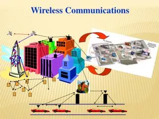
T T Radio Channels Troposcatter Microwave LOS Mobile radio Indoor radio
Two Signal Paths s1(t) s2(t) Received signal r(t) = s1(t) + s2(t) Suppose s1(t) = sin 2f t. Then s2(t) = h s1(t - ) = h sin 2f (t - ) attenuation (e.g., h could be ½) delay (e.g., could be 1 microsec.)
Sinusoid Addition (Constructive) s1(t) r(t) + = s2(t) Adding two sinusoids with the same frequency gives another sinusoid with the same frequency!
Sinusoid Addition (Destructive) s1(t) r(t) + = s2(t) Signal is faded.
Ceiling Hypothetical large indoor environment Indoor Propagation Measurements Normalized received power vs. distance
Power Attenuation distance d reference distance d0=1 Path loss exponent Reference power at reference distance d0 P0 slope (n=2) = -20 dB per decade In dB: Pr = P0 (dB) – 10 n log (d) Pr (dB) slope = -40(n=4) log (d) 0
Large-Scale Path Loss (Scatter Plot) Average Received Power (dBm) Distance (meters)
Shadow Fading • Random variations in path loss as mobile moves around buildings, trees, etc. • Modeled as an additional random variable: Pr = P0 – 10 n log d + X “normal” (Gaussian) probability distribution “log-normal” random variable standard deviation - received power in dB For cellular: is about 8 dB
Large-Scale Path Loss (Scatter Plot) Most points are less than dB from the mean
Empirical Path Loss Models • Propagation studies must take into account: • Environment (rural, suburban, urban) • Building characteristics (high-rise, houses, shopping malls) • Vegetation density • Terrain (mountainous, hilly, flat) • Okumura’s model (based on measurements in and around Tokyo) • Median path loss = free-space loss + urban loss + antenna gains + corrections • Obtained from graphs • Additional corrections for street orientation, irregular terrain • Numerous indoor propagation studies for 802.11
SINR Measurements: 1xEV-DO drive test plots
Link Budget How much power is required to achieve target S/I? • dBs add: Target S/I (dB) + path loss (dB) + other losses (components) (dB) - antenna gains (dB)Total Power needed at transmitter (dB) • Actual power depends on noise level. • Given 1 microwatt noise power, if the transmit power is 60 dB above the noise level then the transmit power is 1 Watt.
Example • Recall that dBm measures the signal power relative to 1 mW (milliwatt) = 0.001 Watt. To convert from S Watts to dBm, use S (dBm) = 10 log (S / 0.001) • Transmitted power (dBm) = -30 + 40 = 10 dBm = 10 mW • What if the received signal-to-noise ratio must be 5 dB, and the noise power is -45 dBm? wireless channel Transmitter Receiver 40 dB attenuation Received power must be > -30 dBm What is the required Transmit power?
Urban Multipath • No direct Line of Sight between mobile and base • Radio wave scatters off of buildings, cars, etc. • Severe multipath
Narrowband vs. Wideband • Narrowband means that the bandwidth of the transmitted signal is small (e.g., < 100 kHz for cellular). It therefore looks “almost” like a sinusoid. • Multipath changes the amplitude and phase. • Wideband means that the transmitted signal has a large bandwidth (e.g., > 1 MHz for cellular). • Multipath causes “self-interference”.
Narrowband Fading Received signal r(t) = h1 s(t - 1 ) + h2 s(t - 2) + h3 s(t - 3 ) + … attenuation for path 1 (random) delay for path 1 (random) If the transmitted signal is sinusoidal (narrowband), s(t) = sin 2f t, then the received signal is also sinusoidal, but with a different (random) amplitude and (random) phase: r(t) = A sin (2f t + ) Received r(t) Transmitted s(t) A, depend on environment, location of transmitter/receiver
Rayleigh Fading Can show: A has a “Rayleigh” distribution has a “uniform” distribution (all phase shifts are equally likely) Probability (A < a) = 1 – e-a2/P0 where P0 is the average received power (averaged over different locations) Ex: P0 =1, a=1: Pr(A<1) = 1 – e-1 = 0.63 (probability that signal is faded) P0 = 1, a=0.1: Pr(A<0.1) = 1 – e-1/100≈ 0.01 (prob that signal is severely faded) Prob(A < a) 1 1-e-a2/P0 a
Small-Scale Fading a = 0.1
Small-Scale Fading • Fade rate depends on • Mobile speed • Speed of surrounding objects • Frequency
Short- vs. Long-Term Fading Short-term fading Long-term fading Signal Strength (dB) T T Time (t) • Long-term (large-scale) fading: • Distance attenuation • Shadowing (blocked Line of Sight (LOS)) • Variations of signal strength over distances • on the order of a wavelength
Combined Fading and Attenuation Received power Pr (dB) distance attenuation Time (mobile is moving away from base)
Combined Fading and Attenuation Received power Pr (dB) distance attenuation shadowing Time (mobile is moving away from base)
Combined Fading and Attenuation Received power Pr (dB) distance attenuation shadowing Rayleigh fading Time (mobile is moving away from base)
Example Diagnostic Measurements: 1XEV-DO drive test measurements drive path
Time Variations: Doppler Shift Audio clip (train station)
Time Variations: Doppler Shift velocity v distance d = v t Propagation delay = distance d / speed of light c = vt/c transmitted signal s(t) delay increases propagation delay received signal r(t) Received signal r(t) = sin 2f (t- vt/c) = sin 2(f – fv/c) t received frequency Doppler shift fd = -fv/c