Download
1 / 160
1.61k likes | 2.07k Vues
Global MHD Simulation with BATSRUS from CCMC. ESS 265 UCLA1 (Yasong Ge, Megan Cartwright, Jared Leisner, and Xianzhe Jia). Outline. Description of Model Global Magnetophere Dayside Magnetopause and Solar Wind Cusp Region Investigation Magnetotail Investigation. BATS-R-US Model.

E N D
Global MHD Simulation with BATSRUS from CCMC ESS 265 UCLA1 (Yasong Ge, Megan Cartwright, Jared Leisner, and Xianzhe Jia)
Outline • Description of Model • Global Magnetophere • Dayside Magnetopause and Solar Wind • Cusp Region Investigation • Magnetotail Investigation
BATS-R-US Model • BATS-R-US, the Block-Adaptive-Tree-Solarwind-Roe-Upwind-Scheme, was developed by the Computational Magnetohydrodynamics (MHD) Group at the University of Michigan, now Center for Space Environment Modeling (CSEM). It was designed using the Message Passing Interface (MPI) and the Fortran90 standard and executes on a massively parallel computer system. • The BATS-R-US code solves 3D MHD equations in finite volume form using numerical methods related to Roe's Approximate Riemann Solver. BATSRUS uses an adaptive grid composed of rectangular blocks arranged in varying degrees of spatial refinement levels. The magnetospheric MHD part is attached to an ionospheric potential solver that provides electric potentials and conductances in the ionosphere from magnetospheric field-aligned currents.
Input parameters and boundary conditions • Fixed Solar Wind velocity of 400km/s, solar wind density of 5X10⁶ protons/m3 and temperature of 1X10⁵. • Two hours initialization with steady southward IMF. • Turning IMF northward for the last two hours. • Default ionosphere without corotation.
Pressure + Velocity vectors t= 00:00 Noon-Midnight meridian view Equatorial view
Pressure + Velocity vectors t= 01:00 Noon-Midnight meridian view Equatorial view
Pressure + Velocity vectors t= 01:58 Noon-Midnight meridian view Equatorial view
Pressure + Velocity vectors t= 02:00 Noon-Midnight meridian view Equatorial view
Pressure + Velocity vectors t= 02:04 Noon-Midnight meridian view Equatorial view
Pressure + Velocity vectors t= 02:06 Noon-Midnight meridian view Equatorial view
Pressure + Velocity vectors t= 02:08 Noon-Midnight meridian view Equatorial view
Pressure + Velocity vectors t= 02:16 Noon-Midnight meridian view Equatorial view
Pressure + Velocity vectors t= 02:30 Noon-Midnight meridian view Equatorial view
Pressure + Velocity vectors t= 02:46 Noon-Midnight meridian view Equatorial view
Pressure + Velocity vectors t= 03:00 Noon-Midnight meridian view Equatorial view
Pressure + Velocity vectors t= 03:16 Noon-Midnight meridian view Equatorial view
Pressure + Velocity vectors t= 03:20 Noon-Midnight meridian view Equatorial view
Pressure + Velocity vectors t= 03:30 Noon-Midnight meridian view Equatorial view
Pressure + Velocity vectors t= 03:46 Noon-Midnight meridian view Equatorial view
Pressure + Velocity vectors t= 04:00 Noon-Midnight meridian view Equatorial view
Plasma temperature t= 00:00
Plasma temperature t= 01:00
Plasma temperature t= 01:58
Plasma temperature t= 02:00
Plasma temperature t= 02:04
Plasma temperature t= 02:06
Plasma temperature t= 02:08
Plasma temperature t= 02:16
Plasma temperature t= 02:30
Plasma temperature t= 02:46
Plasma temperature t= 03:00
Plasma temperature t= 03:16
Plasma temperature t= 03:20
Plasma temperature t= 03:30