Alfred Marshall 1842-1924
350 likes | 743 Vues
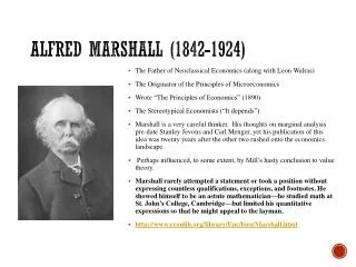
Alfred Marshall 1842-1924. Biographical Details Trained in Mathematics at Cambridge Discovered economics by reading J. S. Mill 1877 Married Mary Paley and both lectured in economics at Bristol 1884 Returned to Cambridge and worked to establish the economics program

Alfred Marshall 1842-1924
E N D
Presentation Transcript
Alfred Marshall1842-1924 • Biographical Details • Trained in Mathematics at Cambridge • Discovered economics by reading J. S. Mill • 1877 Married Mary Paley and both lectured in economics at Bristol • 1884 Returned to Cambridge and worked to establish the economics program • 1890 Principles of Economics • 1919 Industry and Trade
Marshall’s Approach • Wanted his writing to be accessible to the intelligent layman • Mathematics confined to appendices • Wanted to reconcile Classical, marginalist and historicist ideas • Neoclassical synthesis in theory • Theory and application to industry studies
Marshall’s Approach • Partial equilibrium—looking at one market only with everything else held constant • Contrast with Walras’ general equilibrium approach • Short run/long run distinction—what is held constant varies with the time frame • Static analysis vs biological analogy
Theory of Demand • Law of diminishing marginal utility • Diminishing marginal utility translated directly into terms of price • Diminishing willingness to pay • Demand curve is not formally derived through the conditions for a consumer maximum • In the Marshallian discussion price is usually the dependant variable
Demand Theory • The demand curve is interpreted as a schedule of “Demand Prices” • What is held constant along this demand curve? • Marshall assumes both constant money income and constant real income (constant MU of income) • This rules out any significant income effects • Marshall’s “Law of Demand”
Marshallian Demand Curves As Q increases the consumer’s willingness to pay for additional units declines P P1 P2 D Q1 Q2 Q Changes in Q cause changes in demand price, so P is on the vertical axis
Marshall and the Giffen Good Case • Marshall is aware that the MU of income may be affected by price changes • If a good is inferior and important in the budget a large income effect may create an upward sloping demand curve • Marshall attributes this idea to Robert Giffen and to the demand for bread by English labourers • No evidence that Giffen said this and no evidence that bread was a Giffen good
Elasticity of Demand • Marshall invented the elasticity measure of the responsiveness of demand to changes in price • Percentage or proportionate change in Q demanded divided by the percentage or proportionate change in P • Unit free measure of responsiveness • Elasticity and relationship to total expenditure on the good
Consumer’s Surplus • Marshall interpreted a demand curve as a willingness to pay at the margin curve • Consumer is willing to pay more for the first few units of a good than for subsequent units • If the consumer pays a single price for all units bought then the total willingness to pay for those units will exceed the amount actually paid • This is consumer’s surplus
Consumer’s Surplus P a Consumer’s Surplus b P1 D 0 Q Q1 Total willingness to pay for Q1 = 0abQ1 Amount actually paid = 0P1bQ1 Consumer’s surplus = P1ab
Consumers’ Surplus • Marshall thought Consumers’ surplus would be a vital tool for practical policy appraisal • Problem of aggregation over individuals and of interpersonal comparisons • Can only aggregate and compare if the MU of income is the same for everyone • Marshall argued that provided that on average the MU of income is the same than can aggregate and compare across groups
Marshall on Production • Factors of production: land, labour, capital, and organization • Diminishing returns in agriculture • Diminishing returns can also occur with fixed factors other than land • Increasing returns in industry with concentration of industry in particular localities • Increased productivity in industry due to larger scale of particular firms--increased specialization of labour and machinery • Economies of buying and selling on a large scale
Marshall on Production • Forms of business organization and the problems of maintaining energy and efficiency • Joint stock companies and problems of agency • Distinction between external and internal economies • External economies are economies derived from the general development of an industry (external to individual firms) • Internal economies derived from the size of individual firms (internal to the firm)
Marshall on Production • Tendency to decreasing returns in agriculture and natural resource industries • Tendency to increasing returns in other industries • An increase of labour and capital leads generally to improved organization which increases the efficiency of labour and capital • But limits to the size of particular firms • Biological analogy and the life cycle of firms • Concept of the representative firm--firm with average access to internal and external economies
Cost and Supply • Expenses of production—prices that have to be paid to call forth the required supply of productive factors • Supply price of a good • Firms seek to minimize factor costs—principle of substitution • Importance of time frame—short run and long run • Prime costs and supplementary costs (variable and fixed cost)
Short Run Supply • In the short run the quantity of capital available to the firm is fixed • The price the firm receives has to cover prime costs only • With fixed capital will have diminishing returns so that in short periods increased production will raise the supply price • In the short term any return over prime cost is a “quasi rent”
Short Run Market Supply Curve • SR market supply curve slopes upward • Firms have different levels of cost so at a given price some may be making quasi rents, others just covering prime costs and some may be producing nothing (can’t cover even prime cost) • As price rises firms already in production produce more and previously shut down firms will open up
Short Run Market Equilibrium Assuming competitive conditions P S P* D Q” Q* Q’ Q At Q’ demand price is below supply price And output will be reduced. At Q” demand price exceeds supply price and output will Rise. At Q* demand price = supply price
Marshallian vs Walrasian Adjustment to Equilibrium P S P’ P* D P” Q Q’ Q” Q* Walras: At P’ there is excess supply and price falls until D=S (red arrow) Marshall: At Q” supply price exceeds demand price and quantity supplied will fall until demand and supply prices are equal (blue arrow) Does it matter? Issue of stability
Long Run Equilibrium • In the long run firms can change scale and the size of the industry can change • Marshall thinks in terms of the costs of the representative firm • In long run equilibrium the representative firm must be at least covering total costs (prime plus supplementary) • If this is true then size of the industry will not change although individual firms still going through their life cycles • Long run equilibrium population of firms
Long Run Supply • If the representative firm is not covering total cost the industry will shrink in size • If the representative firm industry is more than normally profitable the industry will grow in size • What happens to the costs of a representative firm as the industry changes in size? • Importance of external economies and diseconomies
Long Run Supply • In industries where external economies dominate, growth in industry size will lower the costs of all firms • Long run industry supply curve will be downward sloping (decreasing cost industry) • If external diseconomies dominate industry growth raises costs for all firms • Long run industry supply curve will be upward sloping (increasing cost industry)
Long Run Supply • If external economies and diseconomies just cancel each other out then the costs of firms will not be affected by industry growth • Long run supply curve will be horizontal (constant cost industry) • Marshall though most industries other than natural resource industries had declining long run costs • What might these external economies consist of? • Reduction in factor cost due to industry growth creating a pool of trained labour in that locality
Long Run Supply Curves S” S’ P Increasing cost LS D” D’ Q S’ P S” Decreasing cost LS D’ D” Q
Importance of Decreasing Cost Case • Decreasing costs due to external not internal economies • Therefore decreasing costs are consistent with continued competition • If decreasing costs were due to internal economies this would result in monopoly • Allows Marshall to concentrate on the competitive case—monopoly an exception • Link to modern literature on endogenous growth
Externalities, Taxes and Subsidies • Marshall argued that only in the case of constant costs did competition result in an optimal allocation of resources • External diseconomies meant that industries grew too large as new entrants did not take account of the increased cost they imposed on others • External economies meant that industries did not grow large enough as potential entrants did not consider the beneficial effects they would have on other firms • Marshall’s argument based on consumers’ surplus measures of welfare
Constant Cost Case P b c LS’ a LS” f e d D Q’ Q” Q Subsidy: LS’ to LS” Cost: acdf Benefit: abdf Cost > Benefit Tax: LS” to LS’ Cost: abdf Benefit: abef Cost > Benefit No case for subsidization or taxation
Increasing Cost Case P LS” b a g j LS’ i c h f D Q e d Subsidy: LS” to LS’ Cost: abci Benefit: jgci Cost > Benefit Tax: LS’ to LS” Cost: jgci Benefit: jgfh Benefit > Cost Case for tax where there are external diseconomies
Decreasing Cost Case b a c j g i LS’ d h LS” D e f Subsidy: LS’ to LS” Cost: jcdh Benefit: abdh Benefit> Cost Tax: LS” to LS’ Cost abdh Benefit: abgi Cost > Benefit Case for subsidizing where there are external economies
Monopoly • Marshall’s analysis of monopoly uses average total cost and average revenue curves • Average cost as the monopoly supply price • Monopoly will maximize the difference between demand price and supply price P ATC P* profit D Q Q*
Factor Prices • Critiques both the wage fund theory and the Marxian view that “surplus” is produced by labour • Marginal productivity theory of factor demand • Demand for factors a derived demand • Firm’s demand curve for a factor based on the value of marginal product • On factor supply • Labour supply a function of wages • Supply of capital a function of the interest rate • Producer’s surplus and rent
Factor Markets • Demand and supply explanation of factor prices • Generally assuming competitive factor markets • Concern with the extent of the inequality of the distribution of income • Emphasis on improvement in the quality of labour—training and education to increase productivity • Saw long run possibilities for improvement—cautious reform