Alfred Marshall (1842-1924)

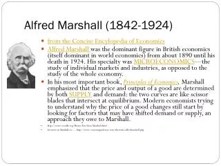
1. Alfred Marshall (1842-1924) • from the Concise Encylopedia of Economics • Alfred Marshall was the dominant figure in British economics (itself dominant in world economics) from about 1890 until his death in 1924. His specialty was MICROECONOMICS—the study of individual markets and industries, as opposed to the study of the whole economy. • In his most important book, Principles of Economics, Marshall emphasized that the price and output of a good are determined by both SUPPLY and demand: the two curves are like scissor blades that intersect at equilibrium. Modern economists trying to understand why the price of a good changes still start by looking for factors that may have shifted demand or supply, an approach they owe to Marshall. • http://www.econlib.org/library/Enc/bios/Marshall.html • for more on Marshall see…. http://www.economyprofessor.com/theorists/alfredmarshall.php

2. Marshall’s contributions • Supply and Demand • Price Elasticity of Demand • Consumer Surplus • Impact of taxation on society • The Short-Run and Long-Run • Optimization • Marshall also taught John Maynard Keynes. If you have taken macroeconomics you have been exposed to the work of Keynes.

3. The Marshallian Method • Step One: Math can be used, but only as a “shorthand language.” • Step Two: Any math should be translated into words. • Step Three: A theory should be illustrated by examples that are “important in real life.” • Step Four: With words and real world illustrations in hand, you can now “burn the mathematics.” • Step Five: If you cannot find any real world examples, burn the theory. • Marshall’s Lesson: Analysis must relate to the world we observe.

4. Deduction vs. induction Deduction: a method of reasoning in which on deduces a theory based on a set of almost self-evident principles. Induction: a method of reasoning in which one develops general principles by looking for patterns in the data. Abduction: a method of analysis that uses a combination of inductive and deductive methods.

5. More on deduction and induction • The basic microeconomic theory of the firm – which we are about to review – is an example of deduction. • Estimating a firm’s demand function is an example of induction. • Interpreting a demand function is an example of abduction – since one needs to understand both data analysis and economic theory to make sense of the empirical results.

6. Maximizing the Value of the Firm • Profit = Total Revenue – Total Cost • The value of the firm is impacted by • Total Revenue.... which is a function of marketing strategies, pricing and distribution policies, nature of competition.... • Total Cost .... which is a function of the price and availability of inputs, alternative production methods... • The model of the firm is a deductive exercise designed to describe both factors that determine profit. • We begin with some basic definitions…

7. Total, Average, and Marginal RelationsDefinitions • Marginal – change in a dependent variable caused by a one unit change in an independent variable. A Marginal Change is represented as ΔY / ΔX • Alternative definitions: • Rate of change • Slope

8. Graphing Total, Marginal, and Average Relations • Slope – a measure of the steepness of a line. OR The rate of change The marginal relation • Tangent – a line that touches but does not intersect a given curve. • This is used to find the slope of a nonlinear curve. • Inflection Point – a point of maximum slope.

9. Examples of Marginal Relationships • Marginal Revenue – change in total revenue associated with a one-unit change in output. • Marginal Cost – Change in total cost associated with a one-unit change in output. • Marginal Profit – Change in profit associated with a one-unit change in output.

10. Examples of Average Relationships • Average Revenue = Total Revenue/Output • What is another name for average revenue? • Average Cost = Total Cost/Output • Average Fixed Cost = TFC / Q • Average Variable Cost = TVC/Q • Average Profit = Total Profit/ Output

11. Review of Basic Microeconomics • Law of Demand – As the price of a good rises, quantity demand will fall, ceteris paribus. • In equation form: P = a – bQ • Total Revenue = Price * Quantity • In equation form: TR = P*Q • OR TR = aQ – bQ2

12. Review of Basic Microeconomics • Revenue Maximization – Activity level that generates the highest revenue. • If P = 100 – 2Q, how much should I produce to maximize total revenue? • Marginal Revenue = 100 – 4Q • Total Revenue is maximized when marginal revenue is zero. WHY??? • When Marginal Revenue is positive, Total Revenue is rising. • When Marginal Revenue is negative, Total Revenue is falling. • When Marginal Revenue is zero, Total Revenue is neither rising or falling, therefore it is maximized. • Therefore, total revenue is maximized at 25 units.

13. Review of Basic Microeconomics • What is the objective of the firm? PROFIT MAXIMIZATION • Profit = Total Revenue – Total Cost • To understand profit, you need to understand both revenue and cost. Understanding total revenue begins with the Law of Demand. Understanding total cost begins with the Law of Diminishing Returns.

14. Review of Basic Microeconomics • The Law of Diminishing Returns – As a variable input increases, holding all else constant, the rate of increase in output will eventually diminish. • OR..... As a firm increases its employment of labor, holding capital and all other factors constant, the productivity of each worker hired will eventually diminish. • WHY? Each additional worker has less and less capital to work with. • The Law of Diminishing Returns is the foundation from which we build the relationship between output and total cost, marginal cost, and average cost.

15. Review of Basic Microeconomics • Average Cost Minimization • Why not Total Cost Minimization? • If Marginal Cost is less than Average Cost, Average Cost will be declining. • If Marginal Cost is greater than Average Cost, Average Cost will be increasing. • When MC = AC, Average Cost is Minimized. • THE MATH OF AC MINIMIZATION

16. Review of Basic Microeconomics • Profit = Total Revenue – Total Cost • Marginal Profit = MR – MC • Profit is maximized when marginal profit equals zero. WHY? • When marginal profit is positive (MR>MC), profit is rising. • When marginal profit is negative (MR<MC), profit is falling. • When marginal profit is zero (MR=MC), profit is not rising or falling, it is maximized.

17. The Law of Demand Law of Diminishing Returns Total Cost and Output Marginal Cost and Average Cost AVERAGE COST MINIMIZING LEVEL OF OUTPUT Price and Output via Own-Price Elasticity Total Revenue and Output Marginal Revenue and Output REVENU E MAXIMIZING LEVEL OF OUTPUT Profit = Total Revenue – Total Cost Marginal Profit = Marginal Revenue – Marginal Cost PROFIT MAXIMIZING LEVEL OF OUTPUT