Regression with Autocorrelated Errors
140 likes | 258 Vues
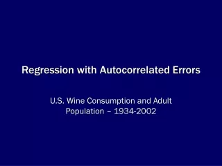
This study analyzes U.S. annual wine consumption (in millions of gallons) against the adult population (in millions) from 1934 to 2002. Utilizing Ordinary Least Squares (OLS) and Generalized Least Squares (GLS) regression techniques, the model examines the relationship between wine consumption and the size of the adult population while accounting for autocorrelated errors. Key metrics include an R-squared value of 0.9324 and significant coefficients for adult population. The analysis provides insights into changing consumption patterns over nearly seven decades.

Regression with Autocorrelated Errors
E N D
Presentation Transcript
Regression with Autocorrelated Errors U.S. Wine Consumption and Adult Population – 1934-2002
Data Description • Y=U.S. Annual Wine Consumption (Millions of Gallons) • X=U.S. Adult Population (Millions of People) • Years – 1934-2002 (Post Prohibition) • Model:
SAS Proc Autoreg Output The AUTOREG Procedure Dependent Variable wine Ordinary Least Squares Estimates SSE 158540.525 DFE 67 MSE 2366 Root MSE 48.64439 SBC 738.318203 AIC 733.84999 Regress R-Square 0.9324 Total R-Square 0.9324 Durbin-Watson 0.1199 Standard Approx Variable DF Estimate Error t Value Pr > |t| Intercept 1 -347.9736 21.9895 -15.82 <.0001 adpop 1 4.3092 0.1417 30.40 <.0001 Estimates of Autocorrelations Lag Covariance Correlation -1 9 8 7 6 5 4 3 2 1 0 1 2 3 4 5 6 7 8 9 1 0 2297.7 1.000000 | |********************| 1 2147.9 0.934807 | |******************* |
SAS Proc Autoreg Output Preliminary MSE 289.8 Estimates of Autoregressive Parameters Standard Lag Coefficient Error t Value 1 -0.934807 0.043717 -21.38 Yule-Walker Estimates SSE 18516.1612 DFE 66 MSE 280.54790 Root MSE 16.74956 SBC 596.454422 AIC 589.752103 Regress R-Square 0.5702 Total R-Square 0.9921 Durbin-Watson 1.6728 Standard Approx Variable DF Estimate Error t Value Pr > |t| Intercept 1 -347.2297 74.0420 -4.69 <.0001 adpop 1 4.2540 0.4546 9.36 <.0001