Download
1 / 22
220 likes | 371 Vues
Using Pictorial Structures to Identify Proteins in X-ray Crystallographic Electron Density Maps. Frank DiMaio dimaio@cs.wisc.edu Jude Shavlik shavlik@cs.wisc.edu George N. Phillips, Jr. phillips@biochem.wisc.edu ICML Bioinformatics Workshop 21 August 2003. Task Overview. . Given

E N D
Using Pictorial Structures to Identify Proteins in X-ray Crystallographic Electron Density Maps Frank DiMaio dimaio@cs.wisc.edu Jude Shavlik shavlik@cs.wisc.edu George N. Phillips, Jr. phillips@biochem.wisc.edu ICML Bioinformatics Workshop 21 August 2003
Task Overview • Given • Electron density for a region in a protein • Protein’s topology • Find • Atomic positions of individual atoms in the density map
Pictorial Structures A pictorial structure is… a collection of image parts together with… a deformable conformation of these parts
v1 v2 v4 v5 Pictorial Structures Formally, a model consists of • Set of parts V={v1, …, vn} • Configuration L=(l1, …, ln) • Edges eij E, connect neighboring parts vi, vj – Explicit dependency between li, lj – G=(V,E) forms a Markov Random Field • Appearance parameters Ai for each part • Connection parameters Cij for each edge e13 e23 v3 e35 e34 v4 e46 v6
- Σimatchi(li) 1 e Z1 Σi matchi(li) + Σ(vi,vj)E dij(li,lj) - Σ(vi,vj)Edij(li,lj) 1 e Z2 Matching Algorithm Overview • Want configuration L of model Θmaximizing P(L|I,Θ) P(I|L,Θ)· P(L|Θ) P(I|L,Θ) = Πi P(I|li,Θ) = P(L|Θ) = Π (vi,vj)E P(li,lj|Cij) = • Equivalent to minimizing
Linear-Time Matching Algorithm • A Dynamic Programming implementation runs in quadratic time • Requires tree configuration of parts • Felzenszwalb & Huttenlocher(2000) developed linear-timematching algorithm • Additional constraint on part-to-part cost function dij • Basic “Trick”: Parallelize minimization computation over entire grid using a Generalized Distance Transform
Pictorial Structures for Map Interpretation Basic Idea: Build pictorial structure that is able to model all configurations of a molecule • Each part in “collection of parts” corresponds to an atom • Model has low-cost conformationfor low-energy states of the molecule
The Screw-Joint Model • Ideally, we would have cost function = atomic energy • Problem: Impossible to represent atomic energy function using pairwise potentials while maintaining tree-structure • Solution: screw-joint model • Ignore non-bonded interactions • Edges correspond to covalent bonds • Allow free rotation around bonds
αi (βi,γi) vi (xi,yi,zi) (βj,γj) αj vj vj (xj,yj,zj) (xij,yij,zij) Screw-Joint Model Details • Each part’s configuration has six params (x,y,z,α,β,γ) with • (x,y,z) is part’s position • αis part’s rotation (about bond connecting vi and vj) • (β,γ) is part’s orientation vi • Part-to-part cost function dijbased on child’s deviation from ideal • Matching cost function matchi based on 3x3x3 template match
Pictorial Structures for Map Interpretation • Ideally, we would … • Build pictorial structure for the entire protein • Run the matching algorithm to get best layout • However, computationally infeasible • Instead, we use two-phase algorithm that … • computes best backbone trace • computes best sidechain conformation(current focus)
Sidechain Refinement • Assume we have a rough Cα trace of the protein • Nextuse pictorial structure matching to place sidechains • Walk along chain one residue at a time, placing individual atoms Cα, ALA_82 Cα, MET_80 Cα, ARG_81 Cα, PRO_83
N C-1 Cα Cα-1 O-1 C Cβ O N O N+1 N O Cα+1 Sidechain Refinement • Given: • residue type • approximate Cα locations • Find: most likely location for sidechain atoms in the residue • ExampleAlanine Matching algorithm
O N N O N C-1 Cα C Cβ O N+1 Learning Model Parameters N Averaged 3D Template Cα Cβ N Cβ Cα C r= 1.51 θ= 118.4° φ = -19.7° Canonic Orientation r= 1.53 θ= 0.0° φ = -19.3° C Alanine Cα Averaged Bond Geometry
Soft Maximums • Sometimes we may get an optimal match like the one to the right • When this occurs, explore the space of non-optimal solutions via soft maximums in DP • Basic Idea: Take a path with probability inverselyproportional to its cost PREDICTED 1 ACTUAL
Soft Maximums • Figure to the right shows soft maximums • Red molecule eventually found • Annealing increases “softness” until legal structure found • Legal structure may not be “right” PREDICTED 2 PREDICTED 1 ACTUAL
Results • Only sidechain refinement implemented & tested • Experimental Methodology • Assume Cα’s known to within 2Å • Trained on 1.7 Å resolution protein, tested on 1.9 Å resolution protein • Templates built for ALA, VAL, TYR, LYS • Model Parameters • Grid spacing of 0.5 Å within diameter 10 Å sphere • Rotational discretization: • 12 rotational steps • 84 orientations
Sidechain Placement • Compared predicted vs. actual location for 599 atoms on testset protein • 29.9% atoms within 0.5Å • 72.3% atoms within 1.0Å • 93.0% atoms within 2.0Å • Recall 0.5Å grid spacing
Predictive Accuracy Task • We used DP matching score as a predictor of amino acid type • Tested 49 ALA, LYS, TYR, VAL residues • Highest scoring normalized template determined type • 61.2% accuracy (majority classification = 33%)
The Good… • PREDICTEDvs. ACTUAL LYSINE LYSINE TYROSINE VALINE
… and the Bad • PREDICTED vs. ACTUAL LYSINE VALINE ALANINE TYROSINE
Future Work • Implement & integrate backbone tracing algorithm, to create complete two-tiered solution • Better strategies to handle illegal molecule configurations • perturbation of branches involved in collisions • more accurate representation of atomic energy function, e.g. torsion angle • Better match function … make use of previous work? • More tests (larger training set, higher resolution)
Acknowledgements • NLM grant 1T15 LM007359-01 • NLM grant 1R01 LM07050-01 • NIH grant P50 GM64598.