Performance Optimization of HPC Applications on Multi- and Manycore Processors
500 likes | 630 Vues
This presentation delves into the optimization of high-performance computing (HPC) applications across diverse multi-core and many-core architectures, including CPUs, GPUs, and hybrid systems. We address the challenges of achieving peak performance, illustrating quantifiable improvements through techniques such as leveraging multicore designs, software-managed memory hierarchies, and off-node communication. Our analysis focuses on three types of applications: Particle-in-Cell codes, Structured Grid Calculations, and Sparse Iterative Methods, highlighting key strategies and optimizations for effective performance enhancement.

Performance Optimization of HPC Applications on Multi- and Manycore Processors
E N D
Presentation Transcript
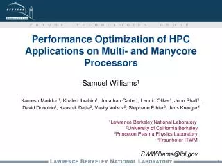
Performance Optimization of HPC Applications on Multi- and ManycoreProcessors Samuel Williams1 Kamesh Madduri1, Khaled Ibrahim1, Jonathan Carter1, Leonid Oliker1, John Shalf1, David Donofrio1, Kaushik Datta2, Vasily Volkov2, Stephane Ethier3, Jens Kreuger4 • 1Lawrence Berkeley National Laboratory 2University of California Berkeley3Princeton Plasma Physics Laboratory3Fraunhofer ITWM SWWilliams@lbl.gov
Introduction • over the last 5 years, a plethora or multicore and accelerator designs have emerged: • CPUs including Core2, Opteron, BlueGene, POWER, SPARC VIIIfx, • GPU accelerator offerings from NVIDIA and ATI • hybrid architectures including IBM’s Cell processor • On paper, (and some benchmarks like LINPACK) they’ve demonstrated impressive peak performance and energy efficiency. • However, optimization of real applications on these architectures can be challenging and ultimately deliver substantially lower than peak performance.
Introduction • In this talk, we explore performance optimization on a variety of architectures include multicore CPUs, GPUs, and Cell processors. • We quantifying the performance and productivity impact of exploiting: • Multicore and heterogeneous architectures • software-managed memory hierarchies • atomic/synchronized operations • off-node communication • We will examine these facets on three classes of applications: • Particle-in-Cell codes • Structured Grid Calculations • Sparse Iterative Methods • Other researchers at NERSC have conducted parallel investigations solely into GPU performance (comparing to out-of-the-box CPU)
Optimization ofParticle-In-Cell (PIC) Codes K. Madduri, K. Ibrahim, S. Williams, E.J. Im, S. Ethier, J. Shalf, L. Oliker, "GyrokineticToroidal Simulations on Leading Mult- and Manycore HPC Systems", Supercomputing (SC), 2011. K. Madduri, E.J. Im, K. Ibrahim, S. Williams, S. Ethier, L. Oliker, "Gyrokinetic Particle-in-Cell Optimization on Emerging Multi- and Manycore Platforms", Parallel Computing, 2011. K. Madduri, S. Williams, S. Ethier, L. Oliker, J. Shalf, E. Strohmaier, K. Yelick, "Memory-Efficient Optimization of Gyrokinetic Particle-to-Grid Interpolation for Multicore Processors", Supercomputing (SC), 2009.
Particle Methods • Naïvely, particle codes iterate on calculation of pairwise forces and moving particles ~ O(N2) computational complexity • Although architecturally efficient (great locality/intensity/comm.), this approach is clearly computationally expensive and intractable for large number of particles • Rather than calculating O(N2) forces, PIC methods calculate O(N) impact of particles on field and O(N) impact of field on particles • particle-to-grid interpolation (scatter-add) • poisson solve • grid-to-particle/push interpolation (gather) • Alternate efficient approaches include • force cut-off methods (assume force=0 beyond a certain range) • particle-tree codes (Barnes Hutt, FMM, Anderson’s Method, etc…)
GyrokineticToroidal Simulations Simulate the particle-particle interactions of a plasma in a Tokamak fusion reactor With millions of particles per processor, the naïve N2 method is totally intractable. Solution is to use a particle-in-cell (PIC) method
GTC Complexity c b d a 2D “Poloidal Plane” r psi 3D Torus zeta mgrid = total number of points The grid is a 3D torus with points uniformly spaced in psi Gyrating particles are approximated via a charged ring. Charge ring is approximated by 4 points Although rings only exist between poloidal planes, their radius can grow to >6% of the poloidal radius.
Typical GTC Structure • Typically, GTC decomposes poloidal planes (typically 64-256) among MPI processes. • Particles sandwiched between a process’ poloidal planes are owned (localized) by that processes. • For additional parallelism, particles may be partitioned and the corresponding poloidal planes replicated • For thread-level parallelism, charge grids can be replicated within a process and particle updates loop-parallelized among threads. • Each time step is composed of 4 major components: • particle to grid interpolation (charge) • poisson solve (poisson/field/smoth) • moving particles (push) • shifting particles among processes (shift) • Typically charge and push dominate the runtime.
charge( ) • charge() is challenged by: • collisions on scatter-increments (need synchronization) • random access patterns to large grid working sets (~36MB per plane) • limited (grid) sequential locality (~256 bits) • low arithmetic intensity (just to stream through particles) • CPU Optimizations: • OpenMP parallelization • static, geometric-based partial grid replication with ghost zones • SIMDized FP atomic-increment (via cmpxchg16b) for particles not in private partition • particle binning • no SIMD intrinsics • GPU Optimizations • keep particles on GPU (accelerator) • cooperative threading on GPUs (to attain coalescing on both particle and grid accesses) • GPU atomic CAS to implement DP atomic increment • binning helps push() but hurts charge() • Sorting updates destroys performance.
charge( ) Partitioned Grid (PG) dramatically accelerates CPU performance over locking solutions Atomics provide an additional boost GPU sorting (thrust) was abysmal GPU CAS helps GPU Coalescing doubles performance If GPUs offered DP increment on par with FxP increment, performance would be on-par with Istanbul
push( ) • push() is challenged by: • random access patterns to large grid working sets (~100MB per plane) • limited (grid) sequential locality (~256 bits) • moderate arithmetic intensity (just to stream through particles) • CPU Optimizations: • NUMA allocation • loop fusion • did not exploit SIMD intrinsics (future work) • GPU Optimizations • keep particles on GPU (accelerator) • heavy optimization of inner kernel • array padding/alignment for coalescing • favor L1 over shared memory, use of texture cache • binning helps push() but hurts charge()
push( ) NUMA and loop fusion (exploiting temporal locality) is essential on CPUs. Loop fusion on GPUs enables further optimizations Favoring L1 (over shared memory) significantly improved GPU performance
shift( ) • shift() is challenged by: • scanning thru particles and removing particles that have left the local domain. • Must then send particles that left to neighboring processes. • Reference implementation is inherently sequential • CPU Optimizations: • threads enumerate private lists of moving particles • track resultant “holes” in particle array • lists are combined and MPI messages sent. • incoming particles fill surplus space first • “Holes” are used when we run out of extra particle space. • GPU Optimizations • Not enough memory for space at end of particle arrays • GPU must express far more parallelism. • As such, thread blocks maintain private buffers in shared memory that are copied (via atomic increments to tail pointers) into the global list when exhausted
Full Application • Integrated optimized routines into full GTC application • Reference (baseline) is best MPI+OpenMP Fortran implementation • Evaluate on: • Intrepid (Blue Gene/P) • Hopper (Cray XE6 MagnyCours) • Intel Nehalem Cluster • Fermi-accelerated Nehalem Cluster • Every platform uses 16 nodes and runs the same “B20” problem • ntoroidal=16, mgrid = 151161 • 20 particles per cell (3M particles per node) • GPU acceleration is handled by offloading shift and push • We keep particles on the GPU • charge grid must be sent to the host for solver • solver sends electric field grids back to the GPU • Does PCIe impede performance?
Performance and Efficiency GPU performance was 34% faster than reference performance However, we were able to accelerate host (Nehalem) performance by 77% GPU increased node power by almost as much as it increased performance (flat energy efficiency)
% Time Intrepid Hopper Intel Cluster Fermi Cluster PCIe time
PIC Summary Efficient threading of CPU implementations reduces memory requirements and eliminates redundancy CPU’s can thus outperform GPUs as well as deliver superior energy efficiency Attaining a cache working set is a challenge on a GPUs given the dynamic gather/scatter operations. CPU’s have ample caches to mitigate this pitfall. Both architectures implemented DP atomic increment via CAS. CPU CAS time is amortized by having a per-thread partial replica. GPU’s have too many threads and too little memory to realize this. PCIe time is not an impediment to GPU performance
Optimization of7- and 27-point stencils constant coefficient, laplacian, single-node, double-precision K. Datta, S. Williams, V. Volkov, J. Carter, L. Oliker, J. Shalf, K. Yelick, "Auto-tuning Stencil Computations on Multicore and Accelerators", in Scientific Computing on Multicore and Accelerators, edited by: JakubKurzak, David A. Bader, Jack Dongarra, CRC Press, 2010, ISBN: 978-1-4398253-6-5.
7-point Stencil z+1 +Z y-1 x+1 x,y,z x-1 y+1 +Y z-1 +X PDE grid stencil for heat equation PDE • Simplest derivation of the Laplacian operator results in a constant coefficient 7-point stencil for all x,y,z: u(x,y,z,t+1) = alpha*u(x,y,z,t) + beta*( u(x,y,z-1,t) + u(x,y-1,z,t) + u(x-1,y,z,t) + u(x+1,y,z,t) + u(x,y+1,z,t) + u(x,y,z+1,t) ) • Clearly each stencil performs: • 8 floating-point operations • 8 memory references all but 2 should be filtered by an ideal cache • 6 memory streams all but 2 should be filtered (less than # HW prefetchers)
7-pt Stencil Performance(full tuning, double-precision, 2563, single node) • CPU optimization was critical to scalability • However, SIMDization was unnecessary (bandwidth) • Orchestrating data movement into LS/shared memory on Cell/GPUs was straightforward • NUMA is important, but can be obviated via MPI process per NUMA node. Hand Optimized CUDA +Cache bypass +Explicit SIMDization +Register Blocking +Cache Blocking +NUMA Reference Implementation
27pt Stencil • Here, we have: • 4 coefficients • 30 flop’s • higher register pressure/reuse • arithmetic intensity of up to 1.875 flops/byte • Subtly performance (stencils/s) can go down (more flops per stencil) but both performance (gflop/s) and time to solution can improve (fewer sweeps to converge) • Two approaches: • 27-point stencil (~30 flops per stencil) • 27-point stencil with inter-stencil common subexpression elimination (~20+ flops/stencil)
27-point Stencil Performance(full tuning, double-precision, 2563, single node) • Clovertown performance wasn’t any worse than 7pt (bandwidth is so poor it’s the bottleneck in either case) • Auto-tuner on a QS22 CBE showed significant boosts. • Cell’s BW begins to obviate optimizations. • hand-optimized version on a GTX280 was probably compute-bound (weak DP) +NUMA +Cache bypass +Explicit SIMDization +Register Blocking +Cache Blocking +Common Subexpression Elimination Reference Implementation
7/27-pt Summary • 7/27-point stencils have • small cache working sets • great spatial locality • great sequential locality • low temporal locality • They can be easily implemented on GPUs/Cell • GPUs deliver modest (~2x) speedups on the kernel. • Communication-avoiding techniques (time skewing, cache oblivious, etc…) can dramatically improve CPU performance. • MPI communication can kill accelerator speedups. • GPU’s 4.5 GStencil/s on 7pt for 2563 is <4ms/sweep • Sustained Infiniband bandwidth is often only 1-2 GB/s • a ghost zone exchange would require 3-6ms • Average performance could be cut by 50-66%
Optimization ofHigh-order Wave Equation inhomogeneous, single-node, single-precision J. Kreuger, D. Donofrio, J. Shalf, M. Mohiyuddin, S. Williams, L. Oliker, F.J. Pfreundt, "Hardware/Software Co-design for Energy-Efficient Seismic Modeling", Supercomputing (SC), 2011.
8th Order Wave Equation(25-point stencil) z+4 +Z z+3 z+2 y-4 y-3 z+1 y-2 x+1 y-1 x+1 x,y,z x+1 x+1 x-1 x-2 y+1 x-3 y+2 x-4 +Y z-1 y+3 y+4 z-2 +X z-3 PDE grid stencil for wave equation PDE z-4 • 8th Order Finite Difference isotropic, inhomogeneous wave equation: for all x,y,z: laplacian = coeff[0]*u[x,y,z,t]; for(r=1;r<=4;r++){ laplacian += coeff[r]*( u[x,y,z+r,t] + u[x,y,z-r,t] + u[x,y+r,z,t] + u[x,y-r,z,t] + u[x+r,y,z,t] + u[x-r,y,z,t] ); } u[x,y,z,t+1] = 2.0*u[x,y,z,t] - u[x,y,z,t-1] + vel[x,y,z,t]*laplacian; • Clearly each 8th order wave equation stencil performs: • 33 floating-point operations • 29 memory references all but 4 should be filtered by an ideal cache • 20 memory streams all but 4 should be filtered
Reference Wave Performance(single node, single-precision, 5123) Baseline on a 2P Nehalem-based Xeon Fermi-accelerated node is 17x faster This is surprising given Fermi only less than 3x the sustained bandwidth as this 2P Nehalem NOTE: no MPI communication
Optimized Wave Performance(single node, single-precision, 5123) Optimizations improved CPU performance by about 5x Some CPU performance has been left on the table GPUs remained 3-4x faster per node MPI communication will mitigate the GPU performance advantage
Energy Efficiency Power and Energy are becoming an increasing constraint on supercomputer scale and cost. Although the Fermi-accelerated node delivers over 3x better performance, it requires 33% more sustained power (and 66% more peak power) Nevertheless, GPUs still offer a 2-3x energy efficiency advantage over current Intel CPUs (ignoring inter-node communication)
Wave Equation Summary • High-order wave equation has • larger cache working sets • higher temporal locality • higher arithmetic intensity • As such, GPU’s higher peak flop/s can be used ~ 3x kernel speedup • Communication-avoiding techniques (time skewing, cache oblivious, etc…) may improve CPU performance (haven’t explore them yet) • MPI communication will mute accelerator speedups. • GPU’s 4.3 GStencil/s is ~30ms/sweep • Ghost zones are 4 (single-precision) elements deep • a ghost zone exchange would require 6-12ms • Average performance could be cut by as much as 30% • GPU’s offer >2.5x speedup, >1.8x energy efficiency over NHM
Optimization of Sparse Iterative Methods S. Williams, N. Bell, J.W. Choi, M. Garland, L. Oliker. R. Vuduc, "Sparse Matrix Vector Multiplication on Multicore and Accelerators", in Scientific Computing on Multicore and Accelerators, edited by: JakubKurzak, David A. Bader, Jack Dongarra, CRC Press, 2010, ISBN: 978-1-4398253-6-5.
Sparse Iterative Methods A x y A.col[ ] ... A.val[ ] for (r=0; r<A.rows; r++) { double y0 = 0.0; for (i=A.rowStart[r]; i<A.rowStart[r+1]; i++){ y0 += A.val[i] * x[A.col[i]]; } y[r] = y0; } ... ... A.rowStart[ ] (a) algebra conceptualization (b) CSR data structure (c) CSR reference code • At the core of most sparse iterative methods is sparse matrix vector multiplication (SpMV) • Evaluate y=Ax • A is a sparse matrix, x & y are dense vectors • Challenges • Very memory-intensive (often <0.166 flops/byte) • Difficult to exploit ILP (bad for pipelined or superscalar), • Difficult to exploit DLP (bad for SIMD)
Auto-tuning SpMV The most important goal is to minimize memory traffic. Typically, we do this by selecting the data representation that minimizes matrix size Register blocking is a common technique that creates small dense blocks within the matrix. Meta data (row/column coordinate) is only stored for each register block as opposed to each nonzero. Alternate matrix formats (COO, CSR, GCSR, etc…) can be combined to minimize total matrix size. We constructed an auto-tuner to explore these and other optimizations on CPUs and Cell. Our collaborators conducted similar experiments on GPUs.
SpMV Performance • Auto-tuner provided moderate speedups on Nehalem and Cell for a range of matrices. (nothing in our toolbox worked for some) • On the GPU, optimization/auto-tuning provided huge speedups • blocked ELLPACK (BELLPACK) did best on many matrices • hybrid (COO+ELLPACK) worked on others.
SpMV Summary Nehalem Naïve OpenMP Nehalem Auto-tuned Pthreads QS22 Auto-tuned Pthreads GTX285 Tuned CUDA Overall, GPU’s delivered better performance for most matrices, often attaining a 2x speedup Cell and Nehalem delivered similar performance. (over last 5 years, IBM’s Cell efforts have been focused in power/cost) Despite the random access challenge, most matrices have sufficiently small working sets that they fit in Fermi’s L2. Unlike PIC, there are no data synchronization challenges. Note, this presumes perfect locality of vectors and matrix within GPU device memory.
Summary • There has been a great deal of fanfare surrounding accelerators • We observe that GPU’s (c2050) offer 2-3x performance advantage over conventional CPU (Nehalem) servers. • many of the applications/kernels of interest tend to be memory intensive • many applications have substantial inter-node MPI requirements • caches benefit complex temporal locality patterns • Adding an accelerator nearly doubles the cost of a node, and increases sustained power by at least 33% (peak by 66%). • CPU and GPU optimization is critical to performance/efficiency • Metrics of Success: • performance per node • performance per $ • performance per Watt
Accelerator Challenges (1) • Random and Dynamic memory access patterns • SW can’t always predict access pattern • trading caches for flops may not be a great idea • trading caches for LS may not be a great idea • Substantial inter-node communication • improved on-node performance coupled with reduced on-node memory results in communication dominated applications = flop/s (or GB/s) vs. GB of capacity • strong scaling among nodes decreases computation per node (also exacerbating the problem) • Finite/diminishing parallelism • strong scaling among nodes decreases computation per node • multigrid (exponentially decreasing work & surface:volume)
Accelerator Challenges (2) • On-chip communication • fastest algorithms communicate data directly between cores • We need arch/programming models that allow this (GPUs/CUDA restricts inter-core communication to cores within a thread block) • fine-grained synchronization can be an impediment (on GPUs, 64b integer increments were 2x faster than CAS) • Accelerator-host communication • push as much computation onto the accelerator as possible • really want manycore processors (not accelerators) • in effect, we may end up turning the host into an accelerator for sequential, OS, and I/O operations
Questions? Acknowledgments Research supported by DOE Office of Science under contract number DE-AC02-05CH11231. This research used resources of the Argonne Leadership Computing Facility at Argonne National Laboratory, which is supported by the Office of Science of the U.S. Department of Energy under contract DE-AC02-06CH11357. 2005.
Three Classes of Locality • Spatial Locality • data is transferred from cache to registers in words. • However, data is transferred to the cache in 64-128Byte lines • using every word in a line maximizes spatial locality. • transform data structures into structure of arrays (SoA) layout • Sequential Locality • Many memory address patterns access cache lines sequentially. • CPU’s hardware stream prefetchers exploit this observation to hide speculatively load data to memory latency. • Transform loops to generate (a few) long, unit-stride accesses. • Temporal Locality • reusing data (either registers or cache lines) multiple times • amortizes the impact of limited bandwidth. • transform loops or algorithms to maximize reuse.
Arithmetic Intensity • True Arithmetic Intensity (AI) ~ Total Flops / Total DRAM Bytes • Some HPC kernels have an arithmetic intensity that scales with problem size (increased temporal locality) • Others have constant intensity • Arithmetic intensity is ultimately limited by compulsory traffic • Arithmetic intensity is diminished by conflict or capacity misses. O( log(N) ) O( 1 ) O( N ) A r i t h m e t i c I n t e n s i t y SpMV, BLAS1,2 FFTs Stencils (PDEs) Dense Linear Algebra (BLAS3) Lattice Methods Particle Methods
Lattice Boltzmann Methods:LBMHD Samuel Williams, Jonathan Carter, Leonid Oliker, John Shalf, Katherine Yelick, "Extracting Ultra-Scale Lattice Boltzmann Performance via Hierarchical and Distributed Auto-Tuning", Supercomputing (SC), 2011. Samuel Williams, Jonathan Carter, Leonid Oliker, John Shalf, Katherine Yelick, "Lattice Boltzmann Simulation Optimization on Leading Multicore Platforms", International Parallel & Distributed Processing Symposium (IPDPS), 2008. Best Paper, Applications Track
25 LBMHD 12 0 23 12 4 25 26 15 15 14 6 2 22 14 8 23 18 18 21 26 24 21 10 9 20 20 22 13 1 13 11 5 24 17 17 16 7 3 16 19 19 +Z +Z +Z +Y +Y +Y +X +X +X macroscopic variables momentum distribution magnetic distribution • Lattice Boltzmann Magnetohydrodynamics (CFD+Maxwell’s Equations) • Used in plasma turbulence simulation • Three macroscopic quantities: • Density, Momentum (vector), Magnetic Field (vector) • Two distributions: • momentum distribution (27 scalar components) • magnetic distribution (15 Cartesian vector components) • Two main functions: • collision( ) = lattice updates = read 73 doubles, 1300 flops, write 79 • stream( ) = MPI ghost zone exchange = 24 doubles per face
LBMHD Stencil Simplified example reading from 9 arrays and writing to 9 arrays Actual LBMHD reads 73, writes 79 arrays
Performance Results(using 2048 nodes on each machine) 1P Quad-core Opteron Node Quad-core Blue Gene/P 2P, 24-core Opteron Node We present the best data for progressively more aggressive auto-tuning efforts Remember, Hopper has 6x as many cores per node as Intrepid or Franklin. So performance per node is far greater. auto-tuning can improve performance ISA-specific optimizations (e.g. SIMD intrinsics) help more Overall, we see speedups of up to 3.4x As problem size increased, so to does performance. However, the value of threading is diminished.
Performance Results(using 2048 nodes on each machine) We present the best data for progressively more aggressive auto-tuning efforts Remember, Hopper has 6x as many cores per node as Intrepid or Franklin. So performance per node is far greater. auto-tuning can improve performance ISA-specific optimizations (e.g. SIMD intrinsics) help more As problem size increased, so to does performance. However, the value of threading is diminished. For small problems, MPI time can dominate runtime on Hopper Threading mitigates this
Performance Results(using 2048 nodes on each machine) We present the best data for progressively more aggressive auto-tuning efforts Remember, Hopper has 6x as many cores per node as Intrepid or Franklin. So performance per node is far greater. auto-tuning can improve performance ISA-specific optimizations (e.g. SIMD intrinsics) help more As problem size increased, so to does performance. However, the value of threading is diminished. For large problems, MPI time remains a small fraction of overall time
Energy Results(using 2048 nodes on each machine) Ultimately, energy is becoming the great equalizer among machines. Hoper has 6x the cores, but burns 15x the power of Intrepid. To visualize this, we explore energy efficiency (Mflop/s per Watt) Clearly, despite the performance differences, energy efficiency is remarkably similar.