Simple Probability Problem
This content delves into probability concepts, particularly the odds of randomly selecting two individuals from a class who are in the same laboratory section. It differentiates between population parameters (true mean, variance, and standard deviation) and sample statistics (sample mean, variance). The text explains the importance of sample representation in statistics, utilizes MATLAB for generating random samples, and provides guidelines for constructing histograms. It emphasizes the role of proper parameter selection in histogram analysis.

Simple Probability Problem
E N D
Presentation Transcript
Simple Probability Problem • Imagine I randomly choose 2 people from this class. What is the probability that both are in the same laboratory section?
(true mean) (sample mean) (sample variance) (true variance) Sample vs Population
Populations Parameters and Sample Statistics • Population parameters include its true mean, variance • and standard deviation (square root of the variance): • Sample statistics with statistical inference can be used • to estimate their corresponding population parameters • to within an uncertainty.
Populations Parameters and Sample Statistics • A sample is a finite-member representation of an • ‘infinite’-member population. • Sample statistics include its sample mean, variance • and standard deviation (square root of the variance):
Normally Distributed Population using MATLAB’s command randtool
The Histogram Figure 7.3 Figure 7.4 Time record Histogram of digital data analog, discrete, and digital signals 10 digital values: 1.5, 1.0, 2.5, 4.0, 3.5, 2.0, 2.5, 3.0, 2.5 and 0.5 V resorted in order: 0.5, 1.0, 1.5, 2.0, 2.5, 2.5, 2.5, 3.0, 3.5, 4.0 V N = 9 occurrences; j = 8 cells; nj = occurrences in j-th cell The histogram is a plot of nj (ordinate) versus magnitude (abscissa).
Proper Choice of Δx High K small Δx The choice of Δx is critical to the interpretation of the histogram. Figure 7.5
Histogram Construction Rules • To construct equal-width histograms: • Identify the minimum and maximum values of x and its range where xrange = xmax – xmin. • Determine K class intervals (usually use K = 1.15N1/3). • Calculate Δx = xrange / K. • Determine nj (j = 1 to K) in each Δx interval. Note ∑nj = N. • Check that nj > 5 AND Δx ≥ Ux. • Plot nj versus xmj,where xmj is the midpoint value of each interval.
Frequency Distribution The frequency distribution is a plot of nj /N versus magnitude. It is very similar to the histogram. Figure 7.7
Histograms and Frequency Distributions in LabVIEW ‘digital’ case ‘continuous’ case