Download
1 / 7
80 likes | 325 Vues
Introduction Monday 21 st 9-10am Turbulence theory Monday 21 st 11-12am Measuring turbulence Monday 28 th 9-10am Modelling turbulence Monday 28 th 11-12am . Marine Turbulence and Mixing. 4 . Modelling turbulence (a brief introduction). Dr. Matthew Palmer

E N D
Introduction Monday 21st 9-10am Turbulence theory Monday 21st 11-12am Measuring turbulence Monday 28th 9-10am Modelling turbulence Monday 28th 11-12am Marine Turbulence and Mixing 4. Modelling turbulence (a brief introduction) Dr. Matthew Palmer matthew.palmer@noc.ac.uk
Turbulence models • Empirical methods: our ability to measure turbulence allows us to identify the true characteristics of turbulence (Nz and Kz) to predict how flow will develop. • But measurements and therefore empirically derived values tend to only have local significance… • …and are difficult to measure. • So we need a method of predicting turbulence in a flow using our knowledge of its characteristics. • This knowledge is derived from observations and experiments but also depending on our generic understanding, so are often termed ‘semi-empirical’.
The TKE turbulent kinetic energy equation and turbulence ‘closure’modelling. A more fundamental way of quantifying all of the turbulent processes that will be useful in general models of vertical turbulent exchange is to use a TURBULENCE CLOSURE SCHEME. The turbulent kinetic energy is described within such a model by: Local rate of change of turbulent kinetic energy (TKE; q2/2) = 1: vertical diffusion of tubulence along the TKE gradient, plus…. 2: local production of turbulence (P) via velocity shear, plus 3: local work done by turbulence against density gradients, plus 4: local dissipation of turbulence, e.
Turbulence closure schemes • Since we are only considering the bulk properties of turbulence, and because turbulence rapidly dissipates, we may often simplify the TKE equation by assuming a local balance between production, buoyancy and dissipation terms. • Since we know turbulence will dissipate in a particular way it is simply parameterised (RHS). • More difficult is predicting the transition to turbulence which is a balance between the terms on the LHS, TKE production and work against buoyancy. • Which is represented by the gradient Richardson number, where B1 = 16.6, is an empirically derived constant (Mellor-Yamada) Where Rig ≤ ¼ somewhere within the flow instability may exist and disturbances may grow (Miles (1961) and Howard (1961) )
Turbulence close scheme The behaviour of turbulence within the model is then described by eddy coefficients dependent on the q and the stability of the flow. The stability functionsSMand SH are calculated based on the local value of the gradient Richardson number, thus relating the eddy coefficients to the local stability. SM, SH Rig 0 Ri= critical (e.g. ¼)
So does it work? • In energetic ‘simple’ flows, such as homogeneous tidal flow, yes • But often small scale processes, particularly during stratification, fails • New ‘parameterisations’ of stratified turbulence have some success • But are still not able to provide a generic solution
summary • Empirically derived turbulent coefficients would enable us to accurately model the ocean. • However turbulence and mixing is highly variable and so measurements have only local significance, and the ocean is BIG and difficult to measure. • So we use semi-empirical ‘turbulence closure schemes’ to estimate how turbulence will behave. • The majority (but not all) TC schemes predict the turbulent coefficients based on the likelihood of instability via stability functions based on the gradient Richardson number. • But we still have a long way to go before we truly understand turbulence and mixing in our oceans.