An Introduction to Statistical Thinking

1. An Introduction to Statistical Thinking January 15, 2014

2. The Omnipresence of Variability • Individuals vary • Repeated measurements on the same individual vary

3. The Omnipresence of Variability • Individuals vary • Repeated measurements on the same individual vary Statistics is a set of ideas and tools that account for variability when dealing with data.

4. Stat Thinking vs. Math Thinking • In pure math, the focus is on abstract patterns. Context is an irrelevant detail. Example: 1, 2, 3, 5, 8, 13, 21, 34, 55, … is an interesting pattern of numbers without context.

5. Stat Thinking vs. Math Thinking • In pure math, the focus is on abstract patterns. Context is an irrelevant detail. • In statistics, whether a pattern is meaningful or interesting depends on context. Example: 3, 5, 23, 37, 6, 8, 20, 22, 1, 3 has seemingly no meaning or interest.

6. The Role of Context Source: George W. Cobb and David S. Moore, Mathematics, Statistics, and Teaching, The American Mathematical Monthly, Vol. 104, No. 9 p. 802

7. What Stat is All About Insight from data in context!

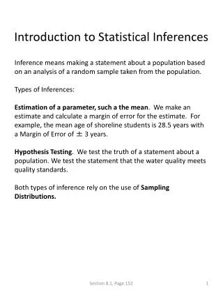
8. The Content of Statistics • Design: where data comes from and how it is gathered • Exploratory data analysis: informal conclusions about data drawn by direct observation • Statistical inference: formal conclusions about unknown parameters drawn indirectly from collected data

9. Break for personal data collection

10. Design • Data are produced in two main ways

11. Design • Data are produced in two main ways • Randomized comparative experiment: Subjects randomly assigned to two groups One group is treated, the other is not (“control”) Responses of two groups are compared

12. Design • Data are produced in two main ways • Randomized comparative experiment: Subjects randomly assigned to two groups One group is treated, the other is not (“control”) Responses of two groups are compared • Observational study: Researchers observe subjects in their natural setting and record variables of interest. Comparisons made among small, homogeneous groups to prevent confounding.

13. Design Examples • Math 109 Personal Info Survey

14. Design Examples • Math 109 Personal Info Survey • The Salk Vaccine Field Trial

15. Design Examples • Math 109 Personal Info Survey • The Salk Vaccine Field Trial • Best and Walker’s smoking and health study

16. Problematic Designs • To study effectiveness of a certain surgery, eligible patients are split into two groups. Those who are too sick to benefit from surgery are put in the control group. The treatment group and control group are compared.

17. Problematic Designs • To determine the effectiveness of a new treatment, a group of patients receive the treatment and are compared to patients treated in other ways in the past (“historical controls”).

18. Quick Quiz • Is the comparison described below from an experiment, an observational study, or neither? Of 8,341 middle-aged men with heart trouble, 5,552 were chosen at random to receive one of five drugs for preventing heart attacks and the rest were assigned to the control group. Subjects who took more than 80% of their prescribed medicine were called “adherers.” For the group assigned to the drug clofibrate, the 5-year mortality rate among adherers was 15%, compared to 25% among non-adherers.

19. Design • Data are produced in two main ways • Randomized comparative experiment • Observational study

20. Design • Data are produced in two main ways • Randomized comparative experiment • Observational study • Experiments often allow causal conclusions, observational studies don’t, even if done during an ongoing experiment.

21. Design • Data are produced in two main ways • Randomized comparative experiment • Observational study • Experiments often allow causal conclusions, observational studies don’t, even if done during an ongoing experiment. • Mathematical models used in statistics are identical for both. Thus context is crucial.

22. Dealing with Data

23. Variables • Characteristics which change from individual to individual

24. Variables • Characteristics which change from individual to individual • Two types • Quantitative: numerical characteristics Examples: Age, family size, income, height

25. Variables • Characteristics which change from individual to individual • Two types • Quantitative: numerical characteristics Examples: Age, family size, income, height • Qualitative/Categorical: non-numerical descriptors Examples: Sex, major, birthplace, marital status

26. Quantitative Variables • Can be discrete or continuous (or both!)

27. Quantitative Variables • Can be discrete or continuous (or both!) • Discrete: values differ by fixed amounts Examples: family size, cars owned

28. Quantitative Variables • Can be discrete or continuous (or both!) • Discrete: values differ by fixed amounts Examples: family size, cars owned • Continuous: difference in values can be arbitrarily small Examples: age, height, weight

29. Quantitative Variables • Can be discrete or continuous (or both!) • Discrete: values differ by fixed amounts • Continuous: difference in values can be arbitrarily small • Discrete variables with large range and small minimum difference may be treated as continuous. Example: income

30. Visualizing Quantitative Data Dot Plot EPA mileage ratings for 100 new cars

31. Visualizing Quantitative Data • Dot plot • Groups values that are the same • Useful for a single discrete variable • Can see individual data points and distribution SPSS: Graphs->Legacy Dialogs->Scatter/Dot Choose Simple Dot Choose X-Axis Variable

32. Histogram

33. Visualizing Quantitative Data • Histogram • Divides data into class intervals • Bars represent proportion of data in each interval • Useful for single continuous or discrete variable • Can see distribution, but not individual data

34. Creating a histogram • Determine class intervals (The widths need not be uniform.)

35. Class Interval Recommendations For discrete quantitative variables, break intervals between data values.

36. Creating a histogram • Determine class intervals • Determine % of data in each interval (Data falling on the boundary of two intervals go in the higher interval.)

37. Creating a histogram • Determine class intervals • Determine % of data in each interval • Determine height of block Height of block = Vertical axis units are “% per (horizontal axis unit)” This scale is called the density scale.

38. Measures of Center Quantitative descriptions of data

39. Mean (average) • Sum of the data values divided by number of data values. • “Balances” a histogram made from the data • May not be a good notion of “middle” if there are a few extreme values • Mean of histogram data is estimated by weighted average.

40. Median • The middle data value when data are ordered smallest to largest. • If there are an even number of data values, the median is the average of the middle two. • Greater than or equal to half of the data, less than or equal to the other half. • Useful when extreme values have reduced importance.

41. Mode • The data value(s) appearing most frequently • Can be more than one (bimodal distribution) • Shows where data tend to concentrate • The only measure of center we’ll discuss that makes sense for a qualitative variable.

42. In SPSS • Analyze => Descriptive Statistics => Frequencies => Statistics

43. The Shape of a Distribution • Skew Right • Long right-hand tail • Mean is larger than median • Skew Left • Long left-hand tail • Mean is smaller than median • Symmetric • Uniform

44. Measures of Variability

45. Range • Difference between largest and smallest data value • Easy to compute, but depends too much on extreme values

46. Interquartile Range (IQR) • The range for the middle 50% of the data • Is not affected by extreme values • To compute IQR of a set of N data values: • Find first quartile (Q1): the 25th percentile data point. • Find third quartile (Q3): the 75th percentile data point. • The IQR = Q3-Q1

47. Standard Deviation (SD) • Measures how far a typical data point is from the mean • Most values (often about 68%) are within one SD of the mean • Very few values (often about 5%) are more than two SDs away from the mean. • The SD has the same units as the data • WARNING: Software computes SD+

48. Calculating SD • Compute deviation for each data value Deviation = data value – mean • Compute root mean square (RMS) of the deviations • Square each deviation • Find the mean of the squared deviations • Take the square root of the result • SD of histogram data is a weighted RMS

49. Why not just take average deviation? • Average absolute deviation • If is replaced by another number, avg. abs. deviation could be smaller. This is not true of SD. • We will see later in the course that • Error in RMS calculations is easier to handle • SD fits best with the theory (Central Limit Theorem)

50. The Normal Approximation