Download
1 / 22
230 likes | 464 Vues
Modeling of Infrasound from the Space Shuttle Columbia Reentry. Robert Gibson and David Norris BBN Technologies Arlington, Virginia, USA Infrasound Technology Workshop La Jolla, California 27-30 Oct 2003 Work sponsored by Air Force Research Laboratory, Contract DTRA01-01-C-0084.

E N D
Modeling of Infrasound from the Space Shuttle Columbia Reentry Robert Gibson and David Norris BBN Technologies Arlington, Virginia, USA Infrasound Technology Workshop La Jolla, California 27-30 Oct 2003 Work sponsored by Air Force Research Laboratory, Contract DTRA01-01-C-0084
Introduction • Space Shuttle Columbia Reentry • STS-107 • 01-Feb-2003 • Loss of orbiter • 1400 UT • 0900 EST • 0600 PST • Nominal trajectory shown • Infrasound observed at multiple arrays in North America
Columbia Investigation • Purpose of this presentation • Explain the infrasound modeling conducted by BBN • Present example results • US Infrasound Working Group formed Feb 2003 • Part of the US DoD Columbia Investigation Support Team • In support of NASA investigation • Participants: • US Government: Army Research Lab, Los Alamos National Lab, NOAA Environmental Technology Lab, Naval Research Lab • Industry: BBN Technologies, Center for Monitoring Research (SAIC) • Academia: Univ. of California-San Diego (L2A/Scripps), Univ. of Hawaii (ISLA), Univ. of Mississippi (NCPA) Optical image, showing left wing damage From AFRL, Kirtland AFB
Background • Infrasound from supersonic bodies has been observed: • Bolides • Concorde • Rockets (Apollo, Titan, Ariane, etc.) • Space shuttle launches and reentries • BBN has used 3-d ray tracing to predict infrasound from Space Shuttle launches • Favorable model vs. data comparisons • Orbiter ascent • Solid rocket booster reentry • Ground truth events are of interest for validating or “calibrating” models • Propagation models • Atmospheric characterizations
Shuttle Modeling Approach Example of eigenrays from one point on a launch trajectory to an array location • Source of infrasound is not impulsive, but continuous and moving • Approximate moving source by modeling a series of discrete events, each with appropriate time delay • Use 3-D ray tracing to find eigenrays from points on reentry trajectory to infrasound array • Determine arrival time and azimuth for each eigenray • Combine all predicted eigenray arrivals at each array
Sources of Information • Shuttle reentry trajectory • NASA, based on actual GPS • Propagation model • InfraMAP tool kit (BBN) • Implementation of HARPA 3-d ray tracing • Environmental characterization • Assimilation of climatology with synoptic model output • NRL-G2S (D. Drob, Naval Research Lab) • Observations, for comparison • US and Canadian station operators • Center for Monitoring Research (SAIC)
Columbia Trajectory and Arrays Altitude (km) Trajectory in white Arrays in red CPA’s in yellow
Examples of Model Results • Results are shown for representative arrays • Short range (in sonic boom carpet) • Medium range (100 – 1000 km) • Long range (> 1000 km) • Atmospheric profiles along propagation path • Variability along path • Presence or absence of stratospheric duct • Typical ray paths • Azimuth vs. time • Color coded by source location • Apparent velocity vs. azimuth (polar plot) • Color coded by signal arrival time
Environmental Variability - SGAR St. George, UT (CPA range =~ 23 km) Atmospheric Characterizations from D. Drob, NRL
Environmental Variability - TXIAR Lajitas, TX (CPA range =~ 522 km) Atmospheric Characterizations from D. Drob, NRL
Environmental Variability – IS10 Lac du Bonnet, Manitoba (CPA range =~ 1864 km) Atmospheric Characterizations from D. Drob, NRL
Typical Ray Path: SGAR St. George, UT
Typical Ray Paths: TXIAR Lajitas, TX
Typical Ray Paths: IS10 Lac du Bonnet, Manitoba
Polar Plot – TXIAR(data) PMCC analysis of observed data from Garces and Hetzer, U. Hawaii (ISLA), “Summary of infrasonic detections and propagation modeling estimates associated with the Columbia reentry of Februrary 1, 2003,” March 2003
Model vs. Data for Pinon Flat (IS57) Receiver azimuth (deg) gmt (hr:min:sec) Data analysis by BBN using InfraTool; Passband: 1-8 Hz
Conclusions • Model results largely consistent with reentry trajectory • Arrival time • Azimuth • Apparent velocity • Supersonic events with ground truth trajectories represent useful validation sources for infrasound modeling techniques • “Modeling of the effects of atmospheric propagation was fairly successful … but does not account for all of the signal complexity at the more distant stations” • From “Report to the Department of Defense on Infrasonic Re-Entry Signals from the Space Shuttle Columbia (STS-107),” ed. by H. Bass, 04-June-2003