Download
1 / 30
310 likes | 421 Vues
Discover the importance of understanding individual tax compliance decisions, explore how behavioral economics challenges traditional models, and delve into non-expected utility theories. Consider social interactions and prospect theory in tax evasion decisions.

E N D
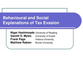
Behavioural and Social Explanations of Tax Evasion Nigar Hashimzade University of Reading Gareth D. Myles University of Exeter Frank Page Indiana University Matthew Rablen Brunel University Financial support from the ESRC/HMRC/HMT is gratefully acknowledged
Introduction • An understanding of the individual tax compliance decision is important for revenue services • Their aim is to design policy instruments to reduce the tax gap • Tax evasion is an area where orthodox analysis has been challenged by behavioural economics • Non-expected utility theory • Social interaction
Standard Model • The probability of being detected is p • Taxpayer chooses declaration X to maximize expected utility max{X} E[U(X)] = [1 – p]U(Yn) + pU(Yc) • Where Yn = Y – tX = [1 – t]Y + tE Yc = [1 – t]Y – Ft[Y – X]= [1 – t]Y – FtE • The sufficient condition for evasion to take place (X < Y) is p < 1/[1 + F]
Standard Model • The evasion decision can be written as max{E} E[U(E)] = [1 – p]U([1 – t]Y + tE) + pU([1 – t]Y – FtE ) • So it follows that E = [1/t]f( . ) • The result that compliance rises as t increases runs counter to "intuition" and has mixed empirical support • Problem of separating aggregate and individual effects • Weakness of experimental evidence
Behavioural Approach • Behavioural economics can be seen as a loosening of modelling restrictions • Two different directions can be taken: (i) Use an alternative to expected utility theory (ii) Reconsider the context in which decisions are taken • The consequences of making such changes are now considered
Non-Expected Utility • There are several non-expected utility models • These have the general form V(X) = w1(p, 1 – p)v(Yc) + w2(p, 1 – p)v(Ync) • w1(p, 1 – p) and w2(p, 1 – p) are translations of p and 1 – p (probability weighting functions) • v(.) is some translation of U(.) • Different representations are special cases of this general form
Prospect Theory • Prospect theory does three things • (i) Translates the probabilities • (ii) Assumes payoff is convex in losses and concave in gains • (iii) Payoffs are measured relative to a reference point, R
Prospect Theory • Yaniv (1999) studies the consequence of paying a tax advance With a tax advance of D • Use Y – D as the reference point • D – tX is the gain if evasion is successful • is the loss if evasion is unsuccessful
Prospect Theory • Observe that D – tX is achieved for sure • So write objective as • Recall that prospect theory has vconvex for losses and concave for gains • Yaniv analyzes the comparative statics of the necessary condition
Prospect Theory • Consider the power function • First assume that D > tY • The next slides illustrates VY for the parameter values Y = 1, t = 0.2, p = 0.1, F = 2, D = 0.3
Prospect Theory • For the power function we can prove: "If there is an interior solution to the first-order condition it must be a minimum" • The same comments (and result) apply to other functional forms • The assumptions of prospect theory combine to create analytical problems
Prospect Theory Two figures for D < tY β = 0.5, γ = 4 p = 0.25, F = 4 p = 0.25, F = 20
Prospect Theory • al-Nowaihi and Dhami (2007) argue that • (i) The reference point should be R = (1 – t)Y • (ii) Standard prospect theory should be used • For this objective it can be shown • A different reference point might change the result
Positive Results • One way to make progress is to assume the probability of detection depends on declared income • Within the prospect theory framework VPT = w⁺(1–p(X))v(t(Y – X)) + w⁻(p(X))v(–Ft(Y – X)) • An appropriate form of p(X) can make the objective strictly concave • Consider the power function of v( ) and p(X) = αp₀X/Y
Positive Results • Now combine the Yaniv model with linear probability pL(X) = α[1 – (1-p₀)(X/Y)] • Advance payment below the true tax liability (D < tY) • t = 0.2, X/Y = 0.74, p = 0.236 • t = 0.3, X/Y = 0.50, p= 0.45 Solid: t = 0.2 Dashed: t = 0.3
Social Interaction • Social interaction allows information to be transmitted through a network • This information affects evasion behaviour by changing beliefs • The network is determined endogenously through choices that are made • The choices are: • Occupation (employed or self-employed) • Level of evasion if self-employed
Occupational Choice • Assume that a choice is made between employment and self-employment • Employment is safe (wage is fixed) but tax cannot be evaded (UK is PAYE) • Self-employment is risky (outcome random) but permits provides opportunity to evade • Selection into self-employment is dependent on personal characteristics
Occupational Choice • A project is a pair {vb, vg} with vb < vg • An individual is described by a triple {w, r,q} • Evasion level is chosen after outcome of project is known • So in state i, i = b, g, Ei solves max EUi = pU((1–t)vi – FtEi) + (1–p)U((1–t) vi+tEi) • The payoff from self-employment is EUs = (1–q) EUb (Eb*) + qEUg (Eg*)
Occupational Choice • Occupational choice compares payoffs from the alternatives • Self-employment is chosen if EUs(q, vb, vg) > Ue(w) • What is the outcome in this setting? • (i) Assume CRRA utility U = Y(1–r)/(1 – r) • (ii) Assume a uniform distribution for (r, q, w)
Occupational Choice • Employment above the locus • Self-employment below the locus • The less risk-averse choose self-employment • But these people will also evade more Employed Self-employed Separation of population p = 0.5, t = 0.25, F = 0.75, vb = 0.5, vg = 2, q = 0.5
Occupational Choice E • The aggregate level of evasion can be increasing in the tax rate • This is the consequence of intensive/extensive margins • The result extends to borrowing to invest t Aggregate evasion E t With borrowing
Social Interaction • A network is a symmetric matrix A of 0s and 1s (bi-directional links) • The network shown is described by 1 2 3 4
Social Interaction • Each period an action is chosen • The network is revised as a consequence of chosen actions • A random selection of meetings occur (a matrix C of 0s, 1s) • Set of permissible meetings is determined by the network (M = A.*C) • At a meeting information is exchanged • Beliefs are updated
Tax Evasion Network • There are n individuals • Individual characteristics {r, w, p, q, vb, vg} are randomly drawn at the outset • A choice is made between e and s • If s is chosen outcome b or g is randomly realised • Given the outcome evasion decision is made • Those in s are then randomly audited
Tax Evasion Network • If audited pi goes to 1 other pi decays pi=d pi, d ≤1 • Type s only meet type s • Links in network evolve as a consequence of choice • Meetings occur randomly between linked individuals • Information on p is exchanged pi = m pi + (1 – m) pj
Results • The model has been run for CRRA utility • n = 1000, t = 100 • r uniform on [0, 10], • True audit probability a= 0.05 • d= 0.95, m= 0.75 • t= 0.25, F = 1.5 p t Mean audit probability (belief)
Results r r t t Self-employed Mean risk aversion Employed Mean risk aversion
Results • The outcome is little changed if decay is increased • Figure uses d= 0.25 • The average belief about audit probability remains high p t
Conclusions • Non-expected utility delivers nothing that is not given by adopting subjective probabilities in the EU model • It requires variable probability to reverse the tax result • Occupational choice selects those who will evade into situations where evasion is possible • Social interaction can lead subjective probability to differ from objective probability