Download
1 / 20
200 likes | 380 Vues
ARTIFICIAL WETLAND MODELLING FOR PESTICIDES FATE AND TRANSPORT USING A 2D MIXED HYBRID FINITE ELEMENT APPROXIMATION Part 2/2. Wanko, A., Tapia, G., Mosé, R., Gregoire, C. Processes. Model. Transport :. Tanks (series or parallel) / Convection-dispersion. PESTICIDES DYNAMICS MODELING.

E N D
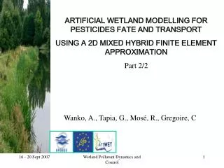
ARTIFICIAL WETLAND MODELLING FOR PESTICIDES FATE AND TRANSPORT USING A 2D MIXED HYBRID FINITE ELEMENT APPROXIMATION Part 2/2 Wanko, A., Tapia, G., Mosé, R., Gregoire, C Wetland Pollutant Dynamics and Control
Processes Model Transport : Tanks (series or parallel) / Convection-dispersion PESTICIDES DYNAMICS MODELING Flow : Mass Balance Concept / Richards Equation Adsorption : Freundlich isotherm / linear distribution Kinetics : Zero order, first order, Michaelis – Menten. Wetland Pollutant Dynamics and Control
2D Discretization : Triangular meshs RT0 Mixte Hybrid Finite Element (MHFE) Numerical method : -Particularly well adapted to the simulation of heterogeneous flow field - The unknown parameters have the same order approximation PESTICIDES DYNAMICS MODELING Unknown parameters : • Pressure head and solute concentrations (edges, mesh center) • Water and transport fluxes through the edges Wetland Pollutant Dynamics and Control
Advection dominant problem : Pe (Peclet number) = Numerical oscillations - Vx ,Vz the pore water velocity in x and z directions, respectively (LT-1 ), - x, z the grid spacing in the x and z direction, respectively (L), - Dxx, Dzz, Dxz the dispersion coefficients (L2 T-1). OSCILLATION CONTROL FOR ADVECTION DOMINANT PROBLEM - FLUX LIMITER In the literature this problem is solve by using : Operator Spliting Technique (OST) + a slope limiting tool (Ackereret al.,1999 ; Siegel et al., 1997 ; Oltean., 2001;Hoteit et al., 2002 ; Hoteit et al., 2004 ) Wetland Pollutant Dynamics and Control
Advection dominant problem : Water fluxes The weight of advection is decreased The weight of advection is increased OSCILLATION CONTROL FOR ADVECTION DOMINANT PROBLEM - FLUX LIMITER A new approche including a flux limiter • Transport fluxes (the previous formulation) • Transport fluxes (the new formulation) [0 ; 1] Wetland Pollutant Dynamics and Control
qr Condition qs Hydrodynamics Ks (cm/d) a (cm-1) Transport n he (cm) Initial 0.1060 0.4686 13.1 0.0104 1.3954 0 Glendale clay loam soil parameter (Kirkland et al., 1992) Boundary Initial and Boundary Conditions One-dimensional Transport verification – The flux limiter Wetland Pollutant Dynamics and Control
a) max Pe=1.02 b) max Pe=1.02x10³ One-dimensional Transport - Flux limiter effect for different Peclet number Wetland Pollutant Dynamics and Control
b) max Pe=1.02x10⁷ One-dimensional Transport - Flux limiter effect for different Peclet number Sensitivity analysis of the parameter a) max Pe = 10.2 b) max Pe=1.02x10³ c) max Pe=1.02x10⁶ Wetland Pollutant Dynamics and Control
Case Vx (m d-1) Vy (m d-1) aL (m2 d-1) aT (m2 d-1) Pe 1 1.0 0.0 1.0 0.1 0.91 2 1.0 0.0 0.1 0.01 7.14 3 1.0 0.0 1x10⁻⁵ 1x10⁻⁶ 7.14x10⁴ Two-dimensional Transport - Flux limiter effect for different Peclet number Parameters used in various cases Two dimensional convection-dispersion problem (left) and regular mesh (right) Wetland Pollutant Dynamics and Control
a) MHFE numerical solution Vx (m d-1) Vy (m d-1) aL (m2 d-1) aT (m2 d-1) b) analytical solution Δx (m) Δy (m) Pe 1.0 0.0 1.0 0.1 1.0 1.0 0.91 X Y Two-dimensional Transport - Flux limiter effect for different Peclet number Case 1 : parameters used Wetland Pollutant Dynamics and Control
Vx (m d-1) Vy (m d-1) aL (m2 d-1) aT (m2 d-1) Δx (m) Δy (m) Pe 1.0 0.0 0.1 0.01 0.5 1.0 7.14 X Y Two-dimensional Transport - Flux limiter effect for different Peclet number Case 2 : parameters used a) MHFE without flux limitingb) MHFE with flux limiting, h = 1c) Analytical solution Iso-concentration lines: second test case Wetland Pollutant Dynamics and Control
Vx (m d-1) Vy (m d-1) aL (m2 d-1) aT (m2 d-1) Δx (m) Δy (m) Pe 1.0 0.0 0.1 0.01 0.5 1.0 7.14 X Y Two-dimensional Transport - Flux limiter effect for different Peclet number Case 3 : parameters used a) MHFE without flux limitingb) MHFE with flux limiting, h = 1c) Analytical solution Iso-concentration lines: second third case Wetland Pollutant Dynamics and Control
: the isotherm linear adsorption coefficient CK is solution concentration of the triangular element K [ML-3], SK is absorbed concentration of the triangular element K [ML-3]. Adsorption model - Verification C(z = 0, t > 0) = 1.0 mg/l C(z , t = 0) = 0.1 mg/l Test case : Kd = 2.38 l/kg (Atrazine ; Vryzas et al., 2007 ) Time (day) Wetland Pollutant Dynamics and Control
C(t = 0, z), the initial concentration, k2 , the dissipation rate, • Zero order k1, the first order rate constant the maximum reaction rate, • First order Km the Michaelis constant X0 the amount of substrate to produce the initial population density • Michaelis – Menten Kinetic models - Verification Simple kinetic models Conditions Wetland Pollutant Dynamics and Control
Kinetic models Initial concentration Kenitic parameters Without kinetic -- Michaelis – Menten Ordre zéro 1er ordre Kinetic models – Verification Initial conditions and kinetic parameters of the tested cases Zero order first orderMichaelis - Menten Wetland Pollutant Dynamics and Control
Depth : 1.5mØ : 3m tank pipe - Sediments («80µ), 30 cm depth, Depth : 2.55mØ : 1m Top layer lysimeter • 12 storage/collector tanks - Fine gravel (4/8), 25 cm depth, - Coarse gravel (10/14), 25 cm depth, Top view Bottom layer Lysimeters : Construction and instrumentation - Model Validation Aim: to elaborate a pilot-constructed wetland design based on bioaugmentation-phytoremediation coupling in order to study and improve the biological potentialities concerning the pesticides remediation CONCEPTION AND DIMENSIONS OF THE PILOT-PLANT • The pilot-plant consists of 12 lysimeters • The filtrating media Phragmites australis, Typha latifolia, Scirpus lacustris • 9 planted bed Wetland Pollutant Dynamics and Control
MATERIAL -12 Lysimeters -flexible feeding pipe -12 collector tanks INPUT -water + pollutant (glyphosate, diuron, copper) Lysimeters : Construction and instrumentation - Model Validation ANALYSES Tests on influents and effluents will be made at different depths Tests on sediments Top view Cross view Wetland Pollutant Dynamics and Control
Lysimeters : Construction and instrumentation - Model Validation ANALYSES Tests on influents and effluents will be made at different depths Tests on sediments Wetland Pollutant Dynamics and Control