Download
1 / 9
220 likes | 952 Vues
Contaminant Fate and Transport. CIVE 7332 Lect 4. Contaminant Transport Equation. C = Concentration of Solute [M/L 3 ] D IJ = Dispersion Coefficient [L 2 /T] B = Thickness of Aquifer [L] C ’ = Concentration in Sink Well [M/L 3 ] W = Flow in Source or Sink [L 3 /T]

E N D
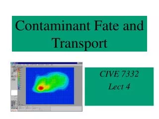
Contaminant Fate and Transport CIVE 7332 Lect 4
Contaminant Transport Equation C = Concentration of Solute [M/L3] DIJ = Dispersion Coefficient [L2/T] B = Thickness of Aquifer [L] C’ = Concentration in Sink Well [M/L3] W = Flow in Source or Sink [L3/T] n = Porosity of Aquifer [unitless] VI = Velocity in ‘I’ Direction [L/T] xI = x or y direction
Analytical Solutions of Equations Closed form solution, C = C ( x, y, z, t) • Easy to calculate, can often be done on a spreadsheet • Limited to simple geometries in 1-D, 2-D, or 3-D • Limited to simple sources such as continuous or instantaneous or simple combinations • Requires aquifer to be homogeneous and isotropic • Error functions (Erf) or exponentials (Exp) are usually involved
Numerical Solution of Equations Numerically -- C is approximated at each point of a computational domain (may be a regular grid or irregular) • Solution is very general • May require intensive computational effort to get the desired resolution • Subject to numerical difficulties such as convergence problems and numerical dispersion • Generally, flow and transport are solved in separate independent steps (except in density-dependent or multi-phase flow situations)
Domenico and Schwartz (1990) • Solutions for several geometries • Generally a vertical plane, constant concentration source. Source concentration can decay. • Uses 1-D velocity (x) and 3-D dispersion (x,y,z) • Spreadsheets exist for solutions. • Dispersion = axvx, where ax is the dispersivity (L) • BIOSCREEN (1996) is handy tool that can be downloaded.
BIOSCREEN Features • Answers how far will a plume migrate? • Answers How long will the plume persist? • A decaying vertical planar source • Biological reactions occur until the electron acceptors in GW are consumed • First order decay, instantaneous reaction, or no decay • Output is a plume centerline or 3-D graphs • Mass balances are provided
Domenico and Schwartz (1990) y Plume at time t Vertical Source x z
Domenico and Schwartz (1990) For planar source from -Y/2 to Y/2 and 0 to Z Y Flow x Z Geometry
Instantaneous Spill in 2-D Spill source C0released at x = y = 0, v = vx First order decay l and release area A 2-D Gaussian Plume moving at velocity V