Download
1 / 33
330 likes | 470 Vues
Andrea Zoia. Fractional dynamics in underground contaminant transport: introduction and applications. Current affiliation: CEA/Saclay DEN/DM2S/SFME/LSET Past affiliation: Politecnico di Milano and MIT MOMAS - November 4-5 th 2008. Outline. CTRW: methods and applications Conclusions.

E N D
Andrea Zoia Fractional dynamics in underground contaminant transport:introduction and applications Current affiliation: CEA/Saclay DEN/DM2S/SFME/LSET Past affiliation: Politecnico di Milano and MIT MOMAS - November 4-5th 2008
Outline • CTRW: methods and applications • Conclusions • Modeling contaminant migration in heterogeneous materials
Transport in porous media • Porous media are in general heterogeneous • Multiple scales: grain size, water content, preferential flow streams, … • Highly complex velocity spectrum • ANOMALOUS (non-Fickian) transport:<x2>~tg • Relevance in contaminant migration • Earlyarrival times (g>1): leakage from repositories • Laterunoff times (g<1): environmental remediation
An example • [Kirchner et al., Nature 2000] Chloride transport in catchments. • Unexpectedly long retention times • Cause: complex (fractal) streams
Main assumption: particles follow stochastic trajectories in {x,t} • Waiting times distributed as w(t) • Jump lengths distributed as l(x) Berkowitz et al., Rev. Geophysics 2006. t x x0 Continuous Time Random Walk
Probability/mass balance (Chapman-Kolmogorov equation) • Fourier and Laplace transformed spaces: xk, tu, P(x,t)P(k,u) CTRW transport equation • P(x,t) = probability of finding a particle in x at time t = = normalized contaminant particle concentration • P depends on w(t) and l(x): flow & material properties • Assume:l(x) with finite std s and mean m ‘Typical’ scale for space displacements
Memory kernel M(u): w(t) ? • Rewrite in direct {x,t} space (FPK): CTRW transport equation • Heterogeneous materials:broad flow spectrum multiple time scales • w(t) ~ t-a-1 , 0<a<2, power-law decay • M(t-t’) ~ 1/(t-t’)1-a : dependence on the past history • Homogeneous materials: narrow flow spectrum single time scale t • w(t) ~ exp(-t/t) • M(t-t’) ~ d(t-t’) : memoryless = ADE
Long time behavior: u0 Asymptotic behavior • The asymptotic transport equation becomes: • Fractional Advection-Dispersion Equation (FADE) • Fractional derivative in time ‘Fractional dynamics’ • Analytical contaminant concentration profile P(x,t)
l(x)~|x|-b-1 , 0<b<2, power law decay Long jumps • Physical meaning: large displacements • Application: fracture networks? • The asymptotic equation is • Fractional derivative in space
Monte Carlo simulation • CTRW: stochastic framework for particle transport • Natural environment for Monte Carlo method • Simulate “random walkers” sampling from w(t) and l(x) • Rules of particle dynamics • Describe both normal and anomalous transport • Advantage: • Understanding microscopic dynamics link with macroscopic equations
Advection and radioactive decay Macroscopic interfaces Breakthrough curves Asymptotic equations Developments Monte Carlo CTRW
P(x,t) Exact CTRW. Asymptotic FADE_ x 1. Asymptotic equations • Fractional ADE allow for analytical solutions • However, FADE require approximations • Questions: • How relevant are approximations? • What about pre-asymptotic regime (close to the source)? • FADE good approximation of CTRW • Asymptotic regime rapidly attained • Quantitative assessment via Monte Carlo
P(x,t) P(x,t) x x FADE* _ Asymptotic FADE_ Exact CTRW. 1. Asymptotic equations • If a 1 (time) or b 2 (space): FADE bad approximation • New transport equations including higher-order corrections: FADE* • Monte Carlo validation of FADE*
Fickian diffusion: equivalent approaches (v = m/<t>) • Center of mass: z(t) ~ t • Spread: S2(t) ~ t P(x,t) S2(t)~t z(t)~t x 2. Advection • Water flow: main source of hazard in contaminant migration • How to model advection within CTRW? • x x+vt (Galilei invariance) • <l(x)>=m (bias: preferential jump direction)
S2(t)~ta S2(t)~t2a z(t)~t z(t)~ta 2. Advection • Anomalous diffusion (FADE): intrinsically distinct approaches P(x,t) P(x,t) x x+vt <l(x)>=m Contaminant migration x x • Even simple physical mechanisms must be reconsidered in presence of anomalous diffusion
Normal diffusion: Advection-dispersion … & decay • Anomalous diffusion: Advection-dispersion … & decay 2. Radioactive decay • Coupling advection-dispersion with radioactive decay
? 3. Walking across an interface • What happens to particles when crossing the interface? • Multiple traversed materials, different physical properties • Two-layered medium • Stepwise changes {s,m,a}1 {s,m,a}2 x Set of properties {1} Set of properties {2} Interface
Analytical boundary conditions at the interface Linking Monte Carlo parameters with equations coefficients 3. Walking across an interface “Physics-based” Monte Carlo sampling rules • Case study: normal and anomalous diffusion (no advection)
Key feature: local particle velocity 3. Walking across an interface P(x,t) layer1layer2 Fickian diffusion layer1layer2 P(x,t) Anomalous x Interface Experimental results Interface x
Breakthrough curve r(t) Outflow t 4. Breakthrough curves • Transport in finite regions Injection B A x0 • Physical relevance: delay between leakage and contamination • Experimentally accessible • The properties of r(t) depend on the eigenvalues/eigenfunctions of the transport operator in the region [A,B]
Space-fractional: transport operator = Fractional Laplacian Open problem… • Numerical and analytical characterization of eigenvalues/eigenfunctions y(x) l r(t) b b x 4. Breakthrough curves • Time-fractional dynamics: transport operator = Laplacian Well-known formalism
Conclusions • Current and future work: link between model and experiments (BEETI: DPC, CEA/Saclay) • Transport of dense contaminant plumes: interacting particles. Nonlinear CTRW? • Strongly heterogeneous and/or unsaturated media: comparison with other models: MIM, MRTM… • Sorption/desorption within CTRW: different time scales? • Contaminant migration within CTRW model
Fractional derivatives • Definition in direct (t) space: • Definition in Laplace transformed (u) space: • Example: fractional derivative of a power
Generalized lattice Master Equation Master Equation Mass conservation at each lattice site s Normalized particle concentration Transition rates Ensemble average on possible rates realizations: Stochastic description of traversed medium Assumptions: lattice continuum
Chapman-Kolmogorov Equation p(x,t) = pdf “just arriving” in x at time t Source terms Contributions from the past history (t) = probability of not having moved P(x,t) = normalized concentration (pdf “being” in x at time t)
Higher-order corrections to FDE FDE: u0 Fourier and Laplace transforms, including second order contributions FDE: k0 FDE Transport equations in direct space, including second order contributions FDE
t Linear CTRW • l(x): how far • w(t): how long x Standard vs. linear CTRW
“Reuse” the remaining portion of the jump in the other layer Start in a given layer Sample a random jump: t~w(t) and x~l(x) The walker crosses the interface The walker lands in the same layer 3. Walking across an interface “Physics-based” Monte Carlo sampling rules
v’’ v’ Dx,Dt Re-sampling at the interface l,w l,w 1 2 x’,t’ v’=x’/t’ Dx Dt=Dx/v’ x’ = L-1(Rx), t’ = W-1(Rt) DRx = L(Dx), DRt = W(Dt) Dx = L-1(Rx) - L-1(DRx), Dt = W-1(Rt) - W-1(DRt)
Concentration ratio at the interface: • Mass conservation: P(x,u) 3. Walking across an interface Analytical boundary conditions at the interface
(x/ta)+ (x/ta)+ (x/ta)- (x/ta)- Equal concentrations at the interface Different concentrations at the interface Normal diffusion: M(u)=1/t Equal velocities: (s/t)+=(s/t)- Boundary conditions Anomalous diffusion: M(u)=u1-a/ta Equal velocities:(s/ta)+=(s/ta)- and a+=a- Local particle velocity Monte Carlo simulation: Local velocity: v=x/ta
df Schramm-Loewner Evolution 5. Fractured porous media • Experimental NMR measures [Kimmich, 2002] • Fractal streams (preferential water flow) • Anomalous transport • Develop a physical model • Geometry of paths
r(t) • Both behaviors observed in different physical contexts CTRW Our model t 5. Fractured porous media • Compare our model to analogous CTRW approach [Berkowitz et al., 1998] • Identical spread <x2>~tg (g depending on df) • Discrepancies in the breakthrough curves • Anomalous diffusion is not universal • There exist many possible realizations and descriptions