What is a model
What is a model. Some notations Independent variables: Time variable: t, n Space variable: x in one dimension (1D), (x,y) in 2D or (x,y,z) in 3D State variables or dependent variables: is a scalar or vector valued variables, generally a function of the independent variables

What is a model
E N D
Presentation Transcript
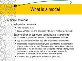
What is a model • Some notations • Independent variables: • Time variable: t, n • Space variable: x in one dimension (1D), (x,y) in 2D or (x,y,z) in 3D • State variables or dependent variables: is a scalar or vector valued variables, generally a function of the independent variables • u(t): the total capital invested; w(t): total dividend to the shareholders • Parameters: The parameters are physical quantities that characterize the physical system to be modeled. These quantities can be defined either in a dimensional or in a dimensionless form and can be obtained either by direct measurements on the system itself or by comparisons between the predictions of the model and the behavior of the real system. • c: speed of light; g: gravitational acceleration; profit rate, ….
What is a model A mathematical model is an equation, or a set of equations, whose solution provides the time-space evolution of the state variable, that is the physical behavior, in the frame work of the mathematical model, of the related physical system. The equation that defines the mathematical model can also be called the state equation
The Process of Mathematical Modeling • Problem identification: The questions to be answered must be clarified. The underlying mechanism at work in the physical situation must be identified as accurately as possible. Formulate the problem in words, and document the relevant data. • Assumptions and physical laws: The must be analyzed to decide which factors are important and which factors are to be ignored so that realistic assumptions can be made. • Model construction or selection: This is the translation of the problem into mathematical language which normally results in a collection of questions and/or inequalities after the variables has been identified. The ``word’’ problem is transformed into an abstract mathematical problem.
The Process of Mathematical Modeling • Model analysis, solution & reduction: The mathematical problem is solved so that the unknown variables are expressed in terms of known quantities, and/or it is analyzed to obtain information about parameters. In some cases, the model may need simplified. • Model interpretation: The solution to the abstract mathematical problem must be compared to the original ``word’’ problem to see if it makes in the real-world situation. If not, go back to formulate more realistic assumptions, and construct a new model. • Model validation, revision & modification: Check whether the solution agrees with the data of the real-world problem. If the correlation is unsatisfactory, return to the ``word’’ problem for a re-appraisal of the data and the assumptions. Modify or add assumptions and construct a new model.
The Process of Mathematical Modeling • Model Implementation: If the solution agrees with the data, then the model can be used to predict what will happen in the future, or conclusions can be drawn to help in future planning, etc. In the case of predictions care should be taken to determine the time interval in which the predictions are valid. • Flow chart of the modelling process identification assumptions and physical laws construction or selection analysis, solution & reduction interpretation validation, revision & modification Implementation
Model classification • No unique classification • Classification by the state variables • Discrete models vs continuous models – state variables depend space variables? • Dynamic model vs static models – state variables depend on time t ??? • Classification by the type of state equation • Algebra model – • ODE models -- • PDE models ---
Model classification • Classification by structure of the state equation • Linear models vs nonlinear models • Classification by parameters and stochasticity • Optimization and/or static models; dynamic models; probability models; …. • Justify a model • Usually use good vs bad (or valid vs invalid) • No absolutely right vs wrong!!! • A model maybe good in some situations & bad otherwise!!
Main focus • Main focus: • How to convert real-world into mathematical models • Basic mathematical analysis techniques • Dimensionless, analytical solutions, steady states, stability, equilibrium, bifurcation, …. • Some basic numerical methods • Not focus • Theory of ODE & PDE, general numerical methods • Some basic knowledge • Calculus, linear algebra, basic physical laws
Another example: World population • World population • Questions: • What is the population in 2020?? • What is the population in 2050???
Malthus’s model • Consider the time interval
Malthus’s model • Malthus’s assumption: • Unlimited resource & no migration • Birth rate and death rate are both constants • The equation
Malthus’s model • Phenomena • Population `explosion’: ``story of Prof. Yanchu Ma’’ • Population distinction • No change • World population
Malthus’s model • Prediction for World population by Malthus’s model • For prediction, we need determine the parameters • Choose two data in the population & set year 1650 as t=0 • Time 1650 (t=0) 1800 (t=150) • Population 0.5 1 • Determine the parameters
World population • Prediction: • Observations: • Under predictions & possible reasons: • Ways to determine parameters!! • Model errors, ……..
Malthus’s model prediction: case 1 • Choose two data in the population • Time 1960 (t0=0) 1970 (t1=10) • Population 1646.40 2074.50 • Determine the parameters • Prediction
Malthus’s model prediction: case 2 • Choose two data in the population • Time 1960 (t0=0) 1980 (t1=20) • Population 1646.40 2413.90 • Determine the parameters • Prediction
Another example: mixing problem • The physical mixing of two species • Chemical system • Biological system • Environmental engineering • A solid material is dissolved in a fluid • Solid is referred as solute; Fluid is referred as solvent • mixture is referred as solution; e.g. salt is dissolved in water • Consider a reservoir or container with inflow and outflow • Inflow: • solution flows into the container at rate (liter of solution /sec: L/s) • Concentrations of the solute (units of mass of solute per unit volume of solution): (kg of solute/ liter of solution: kg/L)
Another example: mixing problem • Outflow: • solution flows out of the container at rate (liter of solution /sec: L/s) • Concentrations of the solute (units of mass of solute per unit volume of solution): (kg of solute/ liter of solution: kg/L) • Solution in the container is kept thoroughly mixed by stirring: uniform mixing • Question: • What is the amount of solute in the container? • What is the concentration of the solute in the container? • Mathematical Model: • Variables: • t : time; : amount of solute in the container • V(t): volume of solution in the container • : concentration of the solute
Another example: mixing problem • Physical law or first principle: mass conservation of solute • Let be infinite small time step and consider time interval • Change of solute in the time interval is: • Change rate:
Another example: mining problem • Initial data: • Rate of change: • First order ODE for time evolution of solute:
Another example: mixing problem • Solution: • A special case: • Simplified first order ODE • Divide both sides by • Integrate both sides over [0,t]
Another example: mixing problem • Solution • Interpretation • Amount of solute decays exponentially with time • Concentration decays exponentially with time • Decay rates are the same • Long time behavior
Another example: mixing problem • Another special case: • Simplified first order ODE • Divide both sides by • Integrate both sides over [0,t]
Another example: mixing problem • Solution
Another example: mixing problem • Interpretation • When inflow is fast than outflow: • Amount of solute and concentration decay with time • Decay rates are different • Long time behavior • When inflow is slower than outflow: • Finite time empty: • Amount of solute and concentration decay with time
Another example: mixing problem • Another special case: • Simplified first order ODE • Solution
Another example: mixing problem • Interpretation • Long time behavior: • When initial concentration is dense: • Amount of solute and concentration decay with time • Decay rates are the same • Dilute process • When initial concentration is dilute: • Amount of solute and concentration increase with time • Increase rates are the same • Pollution process
Another example: mining problem • First order ODE for time evolution of solute: • A special case: • Amount of solute decays exponentially with time • Concentration decays exponentially with time • Decay rates are the same • Long time behavior
Another example: mining problem • Another special case: • Amount of solute and concentration decay with time • Decay rates are different • Long time behavior • Another special case: • Long time behavior: • When initial concentration is dense: • Dilute process • When initial concentration is dilute: • Pollution process
Another example: mixing problem • General case: • Analytical solution in explicit form & interpretation • Non constant inflow and outflow rates: • Analytical solution in integral form & interpretation