Download
1 / 47
470 likes | 583 Vues
By Bharath Sankararaman Tarun V Rajavelu Under Dr.Aidong Zhang. Part I Iterative Clustering of Gene Expression Data for Analyzing Temporal Patterns. Agenda. Microarray – what is it? Gene Expression – what is it? Iterative Clustering Algorithm Motivation Clustering Challenges

E N D
By Bharath Sankararaman Tarun V Rajavelu Under Dr.Aidong Zhang Part IIterative Clustering of Gene Expression Data for Analyzing Temporal Patterns
Agenda • Microarray – what is it? • Gene Expression – what is it? • Iterative Clustering Algorithm • Motivation • Clustering Challenges • Clustering Approach • The algorithm • Measures • Comparison • Conclusion
Microarray • DNA microarray is a collection of microscopic • DNA spots attached to a solid surface, such as • glass, plastic or silicon chip forming an array for the • purpose of expression profiling, monitoring • expression levels for thousands of genes • simultaneously, or for comparative genomic • hybridization
Microarray • The affixed DNA segments are known as probes, thousands of which can be placed in known locations on a single DNA microarray • DNA microarrays can be used to detect RNAs that may or may not be translated into active proteins. This kind of analysis is referred to as "expression analysis“ or expression profiling
Gene Expression • Gene expression, or simply expression, is the process by which a gene's DNA sequence is converted into the functional protein structures of the cell. Non-protein coding genes (e.g. rRNA genes, tRNA genes) are not translated into protein. • The expression of particular genes may be assessed with DNA microarray technology, which can provide a rough measure of the cellular concentration of different messenger RNAs
Iterative Clustering algorithm for Analyzing Temporal Patterns of Gene Expression ~ Seo Young Kim, Jae Won Lee, Jong Sung Bae ~ INTERNATIONAL JOURNAL OF COMPUTATIONAL INTELLIGENCE VOLUME 2 NUMBER 1 2005 ISSN 1304-4508
Motivation • Microarray experiments provide a wealth of information; however, extensive data mining is required to identify the patterns that characterize the underlying mechanisms of action. • For biologists, a key aim when analyzing microarray data is to group genes based on the temporal patterns of their expression levels • Provides insights into genetic capacities and their interactions • Genes with similar functions often evince similar temporal patterns of co-regulation • Due to the large number of genes involved in these experiments and the complexity of biological processes in general, an effective clustering algorithm for grouping genes is crucial to such studies
Clustering challenges • How to determine the number of true clusters ? • How to evaluate samples assigned to those clusters ? • Clustering analysis results rely heavily on limited biological and medical information (i.e. tumor classification), they are not only sensitive to noise but they can also be prone to over-fitting
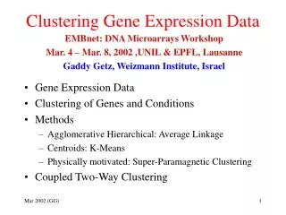
Clustering Approaches • Studies on the analysis of gene expression data have extensively explored the use of unsupervised clustering analysis to find temporal patterns • Resampling and cross-validation methods have been shown to be effective for evaluating the stability of clusters • Consensus clustering method for class discovery - based on a resampling method. Kim et al. devised an extension of consensus clustering that exploits a mixed clustering algorithm based on a mixed distance measure • Here, we introduce a new clustering method based on an iterative algorithm that measures the relative stabilities of clusters from cross-validation criteria
Cross - validation • When a clustering program is created in a supervised situation, it is necessary to be sure that it can perform in an unsupervised situation • In cross-validation, a portion of the data is set aside as training data leaving the remainder as testing data • The quality of performance of the program on the testing data reflects how well it would perform in an unsupervised setting
Approach • One important property of temporal gene expression data is that the data for a given gene at different times may be correlated • Gene expression levels may vary markedly over time • To reflect such time dependencies in observed data, compare the stability and consistency of the results produced by deleting one set of temporal observations at a time • In addition, compare the average expression patterns in each group with the model profiles obtained using our iterative algorithm and existing clustering algorithms
Consensus clustering • The consensus clustering method is a type of resampling-based method • Original data set is perturbed by subsampling iteratively, and then existing clustering methods are iteratively applied to the perturbed data set to construct a distance measure • Data represented as a matrix X = [xgti] • where xgtidenotes expression of the gth gene at time Ti, 1 ≤ i ≤ t
Consensus clustering algorithm • a data resampling scheme and an initial clustering algorithm must be chosen • a similarity matrix is used to assign genes to the proper clusters obtained by applying the algorithm to the various perturbed data sets • ~ where N is the number of genes and Mhis the matrix corresponding to the results obtained by applying the initially selected clustering algorithm to the hth perturbed data set. • ~ Mh(i, j) equals 1 if observations i and j belong to the same • cluster, and 0 otherwise • ~ When all the entries of S are close to 1 or 0, we can infer that • the results have been well clustered. Here, the matrix I − S • represents a distance matrix
Consensus clustering (contd) • When the consensus clustering method is applied to gene expression data to identify temporal patterns, the results obtained depend on the choice of the initial clustering method • To improve the consensus clustering take a mixed similarity matrix to be the average of two similarity matrices, i.e., • Sm= average(S1,S2)
Assessing clusters • Two measures were used to assess and compare the performance of various clustering methods • The average proportion of non-overlap measure computes the average proportion of genes that are not placed in the same cluster by the clustering method under consideration on the basis of the entire data set and the data sets obtained by deleting the expression levels at one time point at a time • The average of the adjusted rand index computes the average degree of agreement between two partitions
Average proportion of non-overlap measure where Cg,i denotes the cluster containing gene g in the clustering based on the data set from which the observations at time Ti have been deleted, and Cg,0 denotes the original cluster containing gene g in the clustering based on the entire data set. A good algorithm is expected to yield a small value of VM1 (K)
Implementation • Agglomerative clustering method UPGMA (Unweighted Pair Group Method with Arithmetic Mean) and the divisive clustering method Diana were used as initial clustering algorithms • Additionally, iterative clustering with UPGMA (ITU), iterative clustering with Diana (ITD), and iterative mixed clustering with UPGMA and Diana were applied • The clustering performance was tested on a real data set and a simulated data set • Publicly available gene expression data set on yeast sporulation was used. The data set consists of expression levels of 6118 genes in the yeast genome measured at seven time points during the sporulation process (i.e., 0, 0.5, 2, 5, 7, 9 and 11.5 hours)
Results of gene expression data For the five clustering algorithms under consideration, computed the two cluster-assessment measures, VM1(K) and VM2(K), over a range of cluster numbers around 7, specifically, K = 4–12. The average proportion of non-overlap measure gave similar results for the five algorithms, although UPGMA and ITU appeared to be the best as judged by this measure. The results for the average of the adjusted rand index on the other hand, indicated that ITU and ITM gave the best performance
Model profile comparison • to classify yeast genes based on their expression levels, Chu et al. hand picked seven small subsets of representative genes using their knowledge of the yeast genome • the same subsets are used to construct the model temporal profiles by averaging the log-expression ratio of all genes in each subset • inspection of the plots for the various algorithms suggests that the ITM plots are closest to the model profiles
Conclusion The iterative algorithms were found to be more accurate and consistent than existing methods. Furthermore, the mixed iterative algorithm gave superior results to the other iterative algorithms tested. The present findings suggest that the mixed iterative algorithm overcomes the demerits of the agglomerative and divisive hierarchical clustering algorithms
Part IIClustering Gene Expression Data Using Graph Theoretic Approach- An Application of Minimum Spanning Trees • MST based Clustering Algorithms
Limitations of well known clustering algorithms- • None of the algorithms (K means, SoM) guaranteed to produce globally optimal solutions for non trivial objective functions. • K means and SoM depend on the ‘regularity’ of the cluster boundaries.
Intution • General 1D problem of grouping n data points to k clusters can be solved by finding k-1 connecting points and “cutting” them. • Here n = 9, k = 3
MST Represntation • Entire gene expression dataset represnted as graph. • MST deduced using Kruskal’s/Prim’s algorithm. • Clusters now become sub trees of this MST. • A multidimensional clustering problem reduced to a tree partitioning problem.
MST Representation of set of data points:- • 2D data points MST
Spanning Tree Representation of a Data Set Let D = {di} be a set of expression data with each di = (e1i, ...., eti) representing the expression levels at time 1 through time t of gene i. We define a weighted (undirected) graph G(D) = (V,E) as follows. The vertex set V = {di|di belongs to D} and the edge set E = {(di, dj)| for di, dj belongs to D and i = j}. Hence G(D) is a complete graph. Each edge (u, v) belongs to E has a weight that represents the distance (or dissimilarity), ρ(u, v), between u and v, which could be defined as the Euclidean distance, the correlational coefficient, or some other distance measures.
Properties of representation. • Let D be a data set and ρ represent the distance between two data points of D.
Algorithm 1 :Clustering through Removing Long MST-Edges • Find the k-1 long edges from the MST and cut them to get clusters. Here the objective function is to minimize the edge distance of all K subtrees. • Approach doesn’t work when intra cluster edges are larger than inter cluster edges. • To determine automatically how many clusters there should be, the algorithm examines the optimal K-clustering for all K = 1, 2, ..., up to some large number to see how much improvement we can get as K goes up. Typically after K reaches the “correct” number (of clusters), the quality improvement levels off,
Iterative Clustering Algorithm • Attempts to partition MST T to k subtrees to optimize a general objective function. • Start with an arbitrary K-partitioning of the tree (selecting K − 1 edges and removing them gives a K-partitioning). Then it repeatedly does the following operation until • the process converges: For each pair of adjacent clusters (connected by a tree edge), go through all tree edges within the merged cluster of the two to find the edge to cut, which globally optimizes the 2-partitioning of the merged cluster, measured by the objective function
Algorithm 3 : A Globally Optimal Clustering • Rather than finding the center point find “representatives” i.e. in addition to partitioning to K sub trees find k data points such that the following objective function is minimized. • Rationale: center may not belong to or even be close to, the data points of its cluster when the shape of the cluster boundary is not convex, which may result in biologically less meaningful clustering results. The representative-based scheme provides an alternative when center-based clustering does not generate desired results.
Algorthim (contd..) • first convert the minimum spanning tree into a rooted tree by arbitrarily selecting a tree vertex as the root. • Define parentchild relationship among all tree vertices. At each tree vertex v, : • S(v, k, d) is defined to be the minimum value of the objective function on the subtree rooted at vertex v, under the constraint that the subtree is partitioned into k subtrees and the representative ofthe subtree rooted at v is d. By definition, the following gives the global minimum of objective function
Uses a dynamic programming (DP) approach to calculate the S() values at each tree vertex v, based on the S() values of v’s children in the rooted MST. • For each v with children, S() of v is calculated as a DP recurrence as follows:
Running time is O(n(2K)s) • K = no of desired clusters • S= max no of children of any tree vertex This global optimization algorithm runs efficiently for a typical clustering problem with a few hundred data points consisting of a dozen or so clusters. It finds the optimal k-clustering for all k’s simultaneously, k ≤ K, for some pre-selected K. For a particular application, if we set K to, say, 30 or to certain percentage of the total number of vertices, we will get the optimal objective values for any k = 1, 2, ....,K. • .
Memetic Algorithms • The combination of an Evolutionary Algorithm with a local search heuristic is called Memetic Algorithm. • Inspired by the notion of a meme – an “adapting” gene. • Difference between memes and genes is that memes are processed and possibly improved by the people that hold them - something that cannot happen to genes. It is this advantage that the memetic algorithm has over simple genetic or evolutionary algorithms. • MAs are known to exploit the correlation structure of the fitness landscape of combinatorial optimization problems.
Pseudocode of a typical MA. • Begin • Initialize population • Local search • Evaluate fitness • While (stopping criteria not met) do • Select individuals for variation • Crossover • Mutation • Local search • Evaluate fitness • Select new population • end
MST-MA Clustering Algorithm • Individual represntation and initialization • Compute MST using Prim’s algorithm • Represent an individual with a bit vector of length n-1, where n = no of genes. 0 - > edge deleted, 1 otherwise. • Cluster memberships can be calculated from MST partition. • To initialize population randomly choose k-1 edges and delete from MST.
Fitness function • Two criteria : • Avoid basing functions on distance to a centroid. • Prefer compact clusters.
Two known objective functions used:- Based on distance from cluster centre- minimizing intra cluster and maximizing intercluster distances. • Authors came up with another function : where in both equations d(·, ·) is the Euclidean distance, |Ci| the number of cluster members in cluster Ci, k the number of clusters and p a term to penalize results including clusters with less than a defined number Ci of members.
Local search • Compute MNVs (mutual neighborhood values). • Edges with higher MNVs might separate two clusters. • for each individual a list of deleted and non-deleted edges is created. During each step, a pair of a deleted and a non-deleted edge is chosen randomly. For the non-deleted edges, edges are favored with a higher mnv and for the deleted edges those with a lower mnv are favored. • Reverse edge states if the resulting clustering has a smaller objective value according to the objective function. • This procedure is repeated until no enhancement could be made or the two lists are empty. Since for each flipped deleted edge a non-deleted edge is flipped as well, the number of clusters is preserved during local search.
Selection, Recombination and Mutation • Selection done for variation and for survival. For variation (recombination and mutation) individuals are randomly selected without favoring better individuals. To determine the parents of the next generation, selection for survival is performed on a pool consisting of all parents of the current generation and the offspring. The new population is derived from the best individuals of that pool. To guarantee that the population contains each solution only once duplicates are eliminated. • The recombination operator is a modified uniform crossover, similar to the uniform crossover for binary strings . To preserve the number of clusters, for both parents, lists of their deleted edges are created. Each bit of the child’s bit vector is set to 1. Then, a pair of deleted edges (one from each parent) is randomly chosen and deleted from the lists. With a probability of 0.5 either the deleted edge of parent a or the one of parent b is copied to the child. This is repeated until both lists are empty. Thus, it is guaranteed that the number of clusters is preserved. • As mutation operator a simple modified point mutation is applied. Since each individual contains much more nondeleted than deleted edges a normal point mutation (just flipping a randomly chosen bit) would lead to more and more clusters. To preserve the number of clusters, again the two lists with deleted and non-deleted edges are created. A pair of a deleted and a non-deleted edge is randomly chosen and both are flipped.
Comparisons done with Best2Partition and AvgLink algorithms. Population size = 40 and termination was done at 200th generation. Recombination and mutation rate was set to 40% Outperforms in terms of both best and average value of objective function and also running time. Comparison
Bibliography • Minimum Spanning Trees for Gene Expression Data Clustering∗ Ying Xu Victor Olman Dong Xu – 2002 Bioinformatics journal. • Clustering Gene Expression Data with Memetic Algorithms based on Minimum Spanning Trees - Nora Speer, Peter Merz, Christian Spieth, Andreas Zell – 2003 IEEE