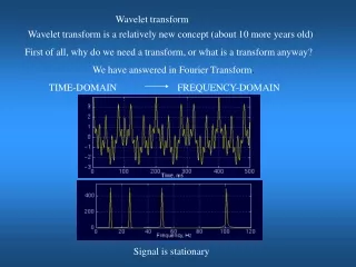
Wavelet Transform
Wavelet Transform . Michael Phipps Vallary S.Bhopatkar. Wavelet Transform . Discrete wavelet transform(DWT) is fast linear operation that operates on a data vector whose length is an integer power of 2, transforming it into a numerically different vector of the same length .

Wavelet Transform
E N D
Presentation Transcript
Wavelet Transform Michael Phipps VallaryS.Bhopatkar
Wavelet Transform • Discrete wavelet transform(DWT) is fast linear operation that operates on a data vector whose length is an integer power of 2, transforming it into a numerically different vector of the same length. • It is invertible and orthogonal: inverse matrix is the simply the transpose of the transform • So DWT can be viewed as rotation in function space, from input space domain to some different domain. • In wavelet domain, the basis functions are known by the names “mother function” and “wavelets”.
The particular kind of dual localization achieved by wavelets renders large classes of functions and operators sparse, or sparse to some high accuracy, when transformed into the wavelet domain. (not clear to me) • Due to advantage of the sparsity , computation becomes faster in wavelet domain. • Unlike Fourier transform, DWT don’t have single unit sets of wavelets.
Daubechies Wavelet Filter Coefficients • Daubechies Wavelets: The set of wavelets was formulated by the Belgian mathematician Ingrid Daubechies in 1988. The formulation is based on the recurrence relation to generate progressively finer discrete samplings of an implicate mother wavelet function. • Daubechies Wavelet Filter Coefficients: • A particular set of wavelets is specified by a particular set of numbers, called wavelet filter coefficients. Here, we will largely restrict ourselves to wavelet filters in a class discovered by Daubechies. The class includes member ranging from highly localized to highly smooth. Most common and highly localizes member called as DAUB4 as it has four coefficient c0, ….., c3
If we multiply above transformation matrix with column vector of data from right, then odd rows convolve the four consecutive data points with filter coefficient c0 ,.., c3. • Even rows perform a different convolution with coefficients c3, -c2, c1, -c0 • Action of matrix: - first perform two convolutions - decimate each of them by half and interleave the remaining halves
c0, …,c3 are called as smoothing filters and represented by H • c3, -c2, c1, -c0 are represented by G and they are not smoothing filters • The c’s are chosen so as to make G yield, insofar as possible, a zero response to a sufficiently smooth data vector. This is done by requiring the sequence c3;c2; c1;c0 to have a certain number of vanishing moments. When this is the case for p moments (starting with the zeroth), a set of wavelets is said to satisfy an “approximation condition of order p.” • This gives the decimated output of H that tells smooth information about the data and output of G gives the detail information of the data • We can reconstruct the original data vector of length N from its N/2 smooth or s-component and its N/2 detail to d component
For the require condition is matrix given by 13.10.1 should be orthogonal i.e. its inverse is nothing but the transposed matrix • 13.10.2 is inverse matrix of 13.10.1 if and only of it satisfies the two equations:
If approximation condition of order p = 2 then we need addition conditions • These (3) and (4) equations are for four unknown coefficients • And its unique solution is given by • If we have six unknown coefficients and p =3 then solutions coefficients are
Discrete Wavelet Transform • In DWT, wavelet coefficient matrix is applied to full data vector of length N • Then it smooth vector to length N/2 and again it smoothen until it reach to trivial number of smooth-…-smooth components. • Therefore the is called “pyramid algorithm”
The endpoint will always be a vector with 2 s and hierarchy of d’s. Once d’s are generated, they are simply propagated through to all subsequent stages • The values of d’s at any stage is called as “wavelet coefficients” and final values of s are called as “mother function coefficients” • DWT is orthogonal linear operator as the full procedure is composition of orthogonal linear operators. • To invert the DWT, one should reverse the procedure mentioned in equation 13.10.7 • The matrices (13.10.1) and (13.10.2) embody periodic (“wraparound”) boundary conditions on the data vector. One normally accepts this as a minor inconvenience: The last few wavelet coefficients at each level of the hierarchy are affected by data from both ends of the data vector. By circularly shifting the matrix (13.10.1) N=2 columns to the left, one can symmetries the wraparound; but this does not eliminate it. It is in fact possible to eliminate the wraparound completely by altering the coefficients in the first and last few rows of (13.10.1), giving an orthogonal matrix that is purely band-diagonal. This variant can be useful when, e.g., the data vary by many orders of magnitude from one end of the data vector to the other (Not conceptually clear)