Understanding Wavelet Transform: A Better Approach to Time-Frequency Analysis in Signal Processing
Learn the limitations of Fourier analysis, the advantages of Gabor's Proposal, and the effectiveness of Wavelet Transform in providing both time and frequency information for signal processing.

Understanding Wavelet Transform: A Better Approach to Time-Frequency Analysis in Signal Processing
E N D
Presentation Transcript
Wavelet Transform PSCI 702 December 7, 2005
Problem with Fourier · Fourier analysis -- breaks down a signal into constituent sinusoids of different frequencies. · A serious drawback in transforming to the frequency domain, time information is lost. When looking at a Fourier transform of a signal, it is impossible to tell when a particular event took place. Time information?
Gabor’s Proposal: Short Time Fourier Transform Requirements: Signal in time domain: require short time window to depict features of signal. Signal in frequency domain: require short frequency window (long time window) to depict features of signal.
FT At Work F F F
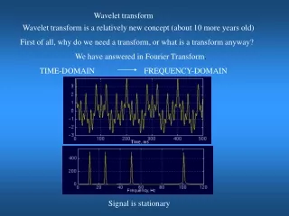
Stationary and Non-stationary Signals • FT identifies all spectral components present in the signal, however it does not provide any information regarding the temporal (time) localization of these components. Why? • Stationary signals consist of spectral components that do not change in time • all spectral components exist at all times • no need to know any time information • FT works well for stationary signals • However, non-stationary signals consists of time varying spectral components • How do we find out which spectral component appears when? • FT only provides what spectral components exist , not where in time they are located. • Need some other ways to determine time localization of spectral components
Stationary and Non-stationary Signals • Stationary signals’ spectral characteristics do not change with time • Non-stationary signals have time varying spectra Concatenation
Non-stationary Signals 50 Hz 20 Hz 5 Hz Perfect knowledge of what frequencies exist, but no information about where these frequencies are located in time
FT Shortcomings • Complex exponentials stretch out to infinity in time • They analyze the signal globally, not locally • Hence, FT can only tell what frequencies exist in the entire signal, but cannot tell, at what time instances these frequencies occur • In order to obtain time localization of the spectral components, the signal need to be analyzed locally • HOW ?
Short Time Fourier Transform (STFT) • Choose a window function of finite length • Put the window on top of the signal at t=0 • Truncate the signal using this window • Compute the FT of the truncated signal, save. • Slide the window to the right by a small amount • Go to step 3, until window reaches the end of the signal • For each time location where the window is centered, we obtain a different FT • Hence, each FT provides the spectral information of a separate time-slice of the signal, providing simultaneous time and frequency information
STFT Frequency parameter Time parameter Signal to be analyzed FT Kernel (basis function) STFT of signal x(t): Computed for each window centered at t=t’ Windowing function Windowing function centered at t=t’
STFT at Work Windowed sinusoid allows FT to be computed only through the support of the windowing function 1 1 0.5 0.5 0 0 -0.5 -0.5 -1 -1 -1.5 -1.5 0 100 200 300 0 100 200 300 1 1 0.5 0.5 0 0 -0.5 -0.5 -1 -1 -1.5 -1.5 0 100 200 300 0 100 200 300
STFT • STFT provides the time information by computing a different FTs for consecutive time intervals, and then putting them together • Time-Frequency Representation (TFR) • Maps 1-D time domain signals to 2-D time-frequency signals • Consecutive time intervals of the signal are obtained by truncating the signal using a sliding windowing function • How to choose the windowing function? • What shape? Rectangular, Gaussian, Elliptic…? • How wide? • Wider window require less time steps low time resolution • Also, window should be narrow enough to make sure that the portion of the signal falling within the window is stationary • Can we choose an arbitrarily narrow window…?
Haar wavelet What are wavelets? · Wavelets are functions defined over a finite interval and having an average value of zero.
What is wavelet transform? · The wavelet transform is a tool for carving up functions, operators, or data into components of different frequency, allowing one to study each component separately. · The basic idea of the wavelet transform is to represent any arbitrary function ƒ(t) as a superposition of a set of such wavelets or basis functions. · These basis functions or baby wavelets are obtained from a single prototype wavelet called the mother wavelet, by dilations or contractions (scaling) and translations (shifts).
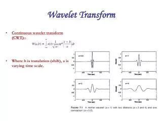
The continuous wavelet transform (CWT) · Fourier Transform FT is the sum over all the time of signal f(t) multiplied by a complex exponential.
· Similarly, the Continuous Wavelet Transform (CWT) is defined as the sum over all time of the signal multiplied by scale , shifted version of the wavelet function : where * denotes complex conjugation. This equation shows how a function ƒ(t) is decomposed into a set of basis functions , called the wavelets. The variables s and tare the new dimensions, scale and translation (position), after the wavelet transform.
· The results of the CWT are many wavelet coefficients, which are a function of scale and position
· The wavelets are generated from a single basic wavelet , the so-called mother wavelet, by scaling and translation: s is the scale factor, tis the translation factor and the factor s-1/2 is for energy normalization across the different scales. · It is important to note that in the above transforms the wavelet basis functions are not specified. · This is a difference between the wavelet transform and the Fourier transform, or other transforms.
·Scale · Scaling a wavelet simply means stretching (or compressing) it.
High frequency low frequency ·Scale and Frequency ·Low scale a Compressed wavelet Rapidly changing details ·High scale a stretched wavelet slowly changing details ·Translation (shift) · Translating a wavelet simply means delaying (or hastening) its onset.
(1) admissibility condition: stands for the Fourier transform of • The admissibility condition implies that the Fourier transform of vanishes at the zero frequency, i.e. · A zero at the zero frequency ( DC component) also means that the average value of the wavelet in the time domain must be zero, must be a wave. Wavelet Properties · This means that wavelets must have a band-pass like spectrum. This is a very important observation, which we will use later on to build an efficient wavelet transform.
Function Representations –Desirable Properties • generality – approximate anything well • discontinuities, nonperiodicity, ... • adaptable to application • audio, pictures, flow field, terrain data, ... • compact – approximate function with few coefficients • facilitates compression, storage, transmission • fast to compute with • differential/integral operators are sparse in this basis • Convert n-sample function to representation in O(nlogn) or O(n) time
Wavelet History, Part 1 • 1805 Fourier analysis developed • 1965 Fast Fourier Transform (FFT) algorithm … • 1980’s beginnings of wavelets in physics, vision, speech processing (ad hoc) • … little theory … why/when do wavelets work? • 1986 Mallat unified the above work • 1985 Morlet & Grossman continuous wavelet transform … asking: how can you get perfect reconstruction without redundancy?
Wavelet History, Part 2 • 1985 Meyer tried to prove that no orthogonal wavelet other than Haar exists, found one by trial and error! • 1987 Mallat developed multiresolution theory, DWT, wavelet construction techniques (but still noncompact) • 1988 Daubechies added theory: found compact, orthogonal wavelets with arbitrary number of vanishing moments! • 1990’s: wavelets took off, attracting both theoreticians and engineers
If j=m and k=n others Discrete Wavelets ·Discrete wavelet is written as j and k are integers and s0 > 1 is a fixed dilation step. The translation factor t0 depends on the dilation step. The effect of discretizing the wavelet is that the time-scale space is now sampled at discrete intervals. We usually choose s0 = 2
· If we look at the scaling function as being just a signal with a low-pass spectrum, then we can decompose it in wavelet components and express it like · admissibility condition for scaling functions · Summarizing once more, if one wavelet can be seen as a band-pass filter and a scaling function is a low-pass filter, then a series of dilated wavelets together with a scaling function can be seen as a filter bank.
The Discrete Wavelet Transform · Calculating wavelet coefficients at every possible scale is a fair amount of work, and it generates an awful lot of data. What if we choose only a subset of scales and positions at which to make our calculations? · It turns out, rather remarkably, that if we choose scales and positions based on powers of two -- so-called dyadic scales and positions -- then our analysis will be much more efficient and just as accurate. We obtain just such an analysis from the discrete wavelet transform (DWT).
Approximations and Details · The approximations are the high-scale, low-frequency components of the signal. The details are the low-scale, high-frequency components. The filtering process, at its most basic level, looks like this: · The original signal, S, passes through two complementary filters and emerges as two signals .
Downsampling · Unfortunately, if we actually perform this operation on a real digital signal, we wind up with twice as much data as we started with. Suppose, for instance, that the original signal S consists of 1000 samples of data. Then the approximation and the detail will each have 1000 samples, for a total of 2000. · To correct this problem, we introduce the notion of downsampling. This simply means throwing away every second data point.
Reconstructing Approximation and Details Upsampling
Wavelet Decomposition Multiple-Level Decomposition The decomposition process can be iterated, with successive approximations being decomposed in turn, so that one signal is broken down into many lower-resolution components. This is called the wavelet decomposition tree.
· Scaling function (two-scale relation) · Wavelet · The signal f(t) can be expresses as DWT
Initialization: · How to calculate DWT given g(m), h(m) and a signal f(m)? Example: f={1,4,-3,0};
Wavelet Reconstruction (Synthesis) Perfect reconstruction :
HL LL HL L H LH HH LH HH original One scale two scales · 2-D Discrete Wavelet Transform · A 2-D DWT can be done as follows: Step 1: Replace each row with its 1-D DWT; Step 2: Replace each column with its 1-D DWT; Step 3: repeat steps (1) and (2) on the lowest subband for the next scale Step 4: repeat steps (3) until as many scales as desired have been completed
Discrete Wavelet Transform • Visual Comparison (a) (b) (c) (a) Original Image256x256Pixels, 24-BitRGB (b) JPEG (DCT) Compressed with compression ratio 43:1(c) JPEG2000 (DWT) Compressed with compression ratio 43:1